Recall that a discrete time system (or map) is defined by a difference equation \[ x_{n+1} = f_\mu(x_n), \qquad\qquad x_n \in \mathbb{R}^n, \] with parameter(s) \(\mu\) (the subscript \(\mu\) may be omitted if no confusion arises). Similar to continuous dynamical system, simple solutions include:
The stability of fixed points or periodic orbits can also be studied via linearisation. If \(x_n\) is close to the fixed point, let \(y_n=x_n-x^*\), then \[ y_n = x_n-x^* = f(x_{n-1})-f(x^*) \approx (x_{n-1}-x^*)f'(x^*) = f'(x^*)y_{n-1}, \] and \(y_n \approx [f'(x^*)]^n y_0\). Therefore, a fixed point \(x^*\) is linearly stable if \(|f'(x^*)| < 1\).
For a periodic orbit with period \(p\), the condition for the fixed points is \[|(f^p)' (x_k)|<1 \qquad \qquad k=0,1,2,\cdots p-1.\] If fact, we only need to check one \(k\), since \((f^p)'(x_0)=(f^p)'(x_1)=\cdots=(f^p)'(x_{p-1})\). Using the chain rule (try the case of \(p=2\) and \(p=3\) to see how it works), \begin{align} \frac{d}{dx} f^p(x_k) &= f'(\underbrace{f(\cdots f(x_k)\cdots)}_{p-1\ \mbox{iterations}}) f'(\underbrace{f(\cdots f(x_k)\cdots)}_{p-2\ \mbox{iterations}}) \cdots f'(x_k) \cr &=f'(x_{k+p-1})f'(x_{k+p-2})\cdots f'(x_k) \cr &=f'(x_{k-1})f'(x_{k-2})\cdots f'(x_k) \cr &=f'(x_0)f'(x_1)\cdots f'(x_{p-1}). \end{align} So there is only one condition for the linear stability of a periodic orbit: \(\prod_{k=0}^{p-1} |f^\prime (x_k) |<1\).
The concept of invariant set can also be defined for maps, but is less used than that for the continuous dynamical systems.
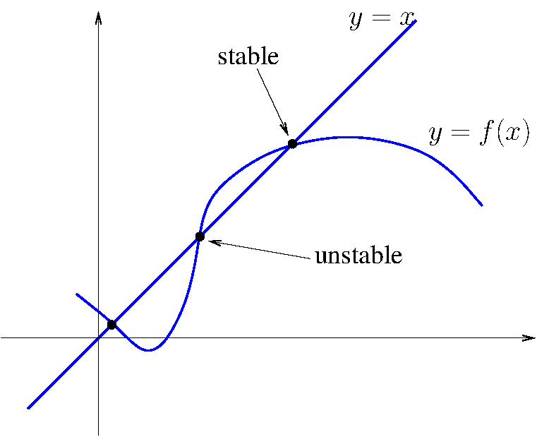
Because of the points \(x_n\) are discrete in space, special graphic tools (other than the phase portrait) are used. First, fixed points for the one dimensional map \(x_{n+1}=f(x_n)\) can be viewed as the intersection of the straight line \(y=x\) and the curve \(y=f(x)\). If \(f'(x^*)\) is positive at the fixed point \(x^*\), the stability can also be determined graphically, by comparing \(f'(x^*)\) with the slope of \(y=x\) (see Figure 6.1).
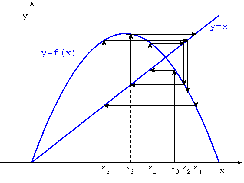
The iteration of the trajectory \(x_0,x_1,\cdots\) can be viewed from the cobweb diagram (right figure in Figure 6.1: (1) the vertical line \(x=x_n\) intersect the curve \(y=f(x)\) at \((x_n,f(x_n))=(x_n,x_{n+1})\); (2) the horizontal line through \((x_n,x_{n+1})\) intersect the line \(y=x\) at \((x_{n+1},f(x_{n+1})\); (3) then the vertical line through \((x_{n+1},x_{n+1})\) becomes \(x=x_{n+1}\) and the whole process can be continued again.
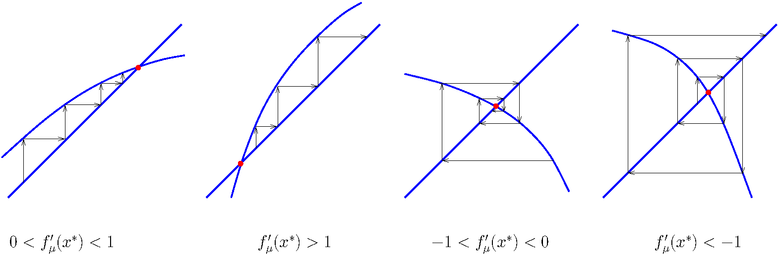
The behaviour of the map \(x_{n+1}=f_\mu(x_n)\) near a fixed point can be understood using the cobweb diagram as shown in Figure 6.2. While the stability (inward towards the fixed point \(x^*\) or not) is determined by whether \(|f_\mu'(x^*)|\) is greater than unit, the sign of \(f_\mu'(x^*)\) determines whether the diagram looks like stairs (\(f_\mu'(x^*)>0\)) or spirals (\(f_\mu'(x^*)<0\)).