In this section, we will study mainly the properties of
linear systems around fixed points, as a first step towards the understanding of
more complicated behaviours of nonlinear
systems. The local, linear part can be obtained from the full nonlinear
counterpart via Taylor expansion around the fixed points.
3.1 Taylor's theorem
Suppose \(x^* \in \mathbb{R}^n\) is a stationary point of \(\dot{x}=f(x)\), that is \(f(x^*)=0\).
If \(z=x-x^*\) is small, we can use
Taylor's Theorem to expand \(f(x)\) around \(x^*\), that is,
\[
\dot{x} = \dot{z} = f(x) = f(x^*+z) = \cancel{f(x^*)}+ D f(x^*)z+O(|z|^2) = Df(x^*)z+O(|z|^2).
\]
Here \(Df(x^*)\) is the \(n\times n\) Jacobian matrix with entries
\(\left[ D f(x) \right]_{ij} = \partial f_i/\partial {x_j} (x)\).
The 'big-O' notation means that if a function \(g(z)=O(|z|^2)\) then
\(\frac{|g(z)|}{|z|^2} < C\), for some \(C<\infty\), on a neighbourhood of \(z=0\). If \(z\) is small then we can hope to ignore the small \(O(|z|^2)\) terms and consider the linearisation about \(x^*\): \(\dot z=Az\) with \(A=D f(x^*)\) or \(A_{ij}=\frac{\partial f_i}{\partial x_j}(x^*)\) .
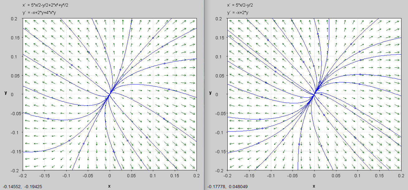
Example 3.1
Consider the system
\begin{align}\label{eq:fullnleq}
\begin{pmatrix} \dot{x} \cr \dot{y} \end{pmatrix}
= f(x,y) = \begin{pmatrix}
\frac{5}{2} x - \frac{1}{2} y + 2 x^2 + \frac{1}{2} y^2\cr
- x + 2 y + 4xy
\end{pmatrix},
\end{align}
for which \((0,0)\) is a stationary point.
Since
\begin{equation*}
D f(x,y) = \begin{pmatrix}
\frac{5}{2} + 4 x & - \frac{1}{2} + y \\
- 1 + 4y & 2 + 4x \\
\end{pmatrix},
\end{equation*}
the system can be approximated by
\[
\qquad\qquad \begin{pmatrix} \dot{x} \cr \dot{y} \end{pmatrix}
= A \begin{pmatrix} x \cr y \end{pmatrix},
\qquad \mbox{where}\quad
A =Df(0,0)= \begin{pmatrix}
\frac{5}{2}& - \frac{1}{2} \\
- 1 & 2 \\
\end{pmatrix}.
\]
which could have been read off directly from the linear part of the
equation (1).
Figure 3.0
The vector field and the trajectories of the full nonlinear system (left) and its
linearised system very close to the origin.
Key questions in the next few subsections
How can we characterize solutions of linear equations \(\dot{x}=Ax\)?
(Harder) How/when does information about the linearisation provide useful local
information about the original (nonlinear) problem?
Example 3.2Consider the system
\begin{equation} \label{eq:lineq2}
\begin{pmatrix} \dot{x} \cr \dot{y} \end{pmatrix}
= \begin{pmatrix} 1 - ax^2 + y \cr bx\end{pmatrix}.
\end{equation}
We start with the stationary points, by looking for zeros
of the right hand side of the system: the second equation implies that
\(x=0\); substituting it back into the first equation, we get \(y=-1\).
Therefore, the only stationary point is \((0,-1)\).
From \(f(x,y)=\begin{pmatrix} 1-ax^2+y \cr bx\end{pmatrix}\),
\({D} f(x,y) = \begin{pmatrix}
-2ax & 1\\ b & 0
\end{pmatrix} \)
and \( {D} f(0,-1) = \begin{pmatrix}
0 & 1\\ b & 0
\end{pmatrix}\).
The linearisation in coordinates
\(
\begin{pmatrix} x \cr y \end{pmatrix}
=
\begin{pmatrix} 0 \cr -1 \end{pmatrix}
+
\begin{pmatrix} u \cr v \end{pmatrix}
\)
is
\(
\begin{pmatrix} \dot{u} \cr \dot{v} \end{pmatrix}
= \begin{pmatrix}
0 & 1\\
b & 0\\ \end{pmatrix}
\begin{pmatrix} {u} \cr {v} \end{pmatrix}
\)
or
\begin{align*}
\dot{u} = v,\qquad
\dot{v} =bu.
\end{align*}
This linsear system can be solved by eliminating \(v\) (or alternatively using matrix exponential):
\(\ddot{u} = \dot{v} = bu\), or \(\ddot{u} - bu = 0\).
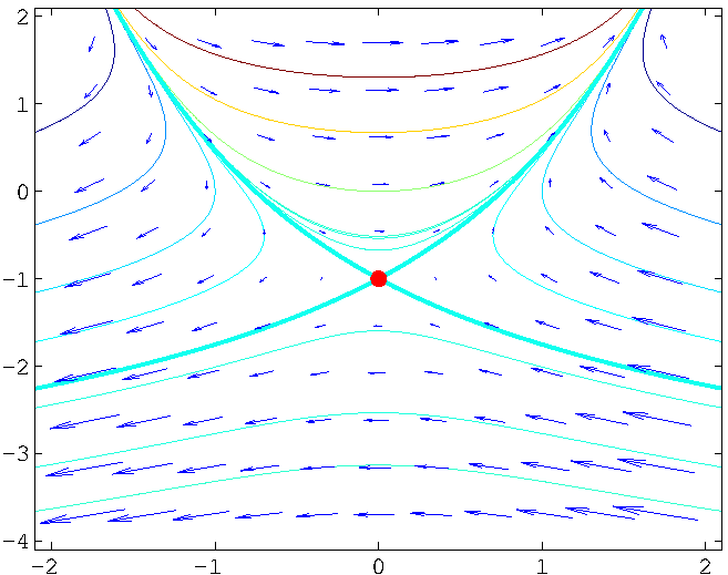
Using elementary methods in ODEs, if \(b>0\) the solutions are
\begin{equation*}
u = A e^{\sqrt{b}t} + B e^{-\sqrt{b}t} \quad
\text{ with } \quad v = \dot{u} = \sqrt{b} (A e^{\sqrt{b}t} - B
e^{-\sqrt{b}t}),
\end{equation*}
for constants \(A\) and \(B\) determined from the initial condition.
Most solutions are unbounded (with general \(A\) and \(B\)). But the special solution with \(A=0\)
converges to the origin.
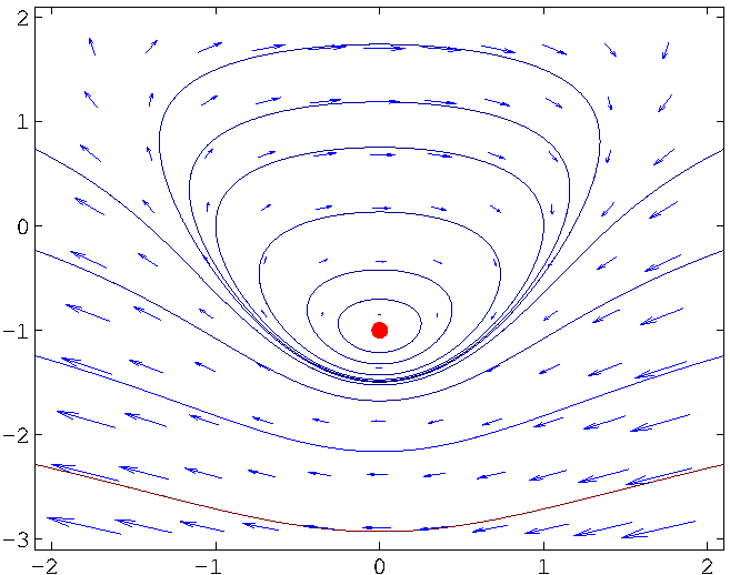
If \(b<0\) then \begin{equation*} u=A \cos \sqrt{|b|} t + B \sin \sqrt{|b|} t \quad \text{ and } \quad v=\sqrt{|b|} \big( -A \sin \sqrt{|b|} t + B \cos \sqrt{|b|} t\big) \end{equation*} i.e. solutions of the linearisation oscillate in time.
Figure 3.1 The phase portrait for two systems: (left figure) \(\dot{x} = 1-x^2+y,\dot{y}=x\)
and (right figure) \(\dot{x}=1-x^2+y,\dot{y}=-x\), with common fixed point \((0,-1)\).
Question: When does this linear analysis give accurate information
about the behaviour of the full nonlinear problem? It will turn out that
the behaviour if \(b>0\) is a good sense of the general behaviour (locally)
whilst this may not be the case if \(b<0\). For instance, the trajectories of the system \(\dot{x}=1-x^2+y,\dot{y}=-x-x^2\) around the fixed point \((0,-1)\) are spirals. For the above system \(\dot{x}=1-ax^2+y,\dot{y}=bx\), you can show that \[ V(x,y)=(2a^2x^2-2a+b-2ay)\exp(2ay/b) \] is conserved under the full system (2), and the trajectories are governed by \(V(x,y)=C\) for different constants \(C\).
Consider the previous example with \(a=1\), so that the sysmtem becomes
\[
\dot{x} = 1-x^2+y,\quad
\dot{y} = bx.
\]
Move the slider to change the value of \(b\), and see how the qualitative behaviour of the system changes as \(b\) crosses the value zero, especially for points
starting on the positive \(y\)-axis. The sensitive dependence of the behaviour when the parameter is changed around a particular value is called bifurcation, the topic
of Chapter 6.