The only `typical' case not treated in the previous section is the
appearance of purely imaginary (simple) eigenvalues \(\pm i\omega\),
instead of zero eigenvalues. Usually, there is only one zero eigenvalue (as seen in
all examples in the previous section), and the centre manifold is only one dimension.
But in the simplest case with bifurcation with two purely imaginary eigenvalues,
the centre manifold at \(\mu=0\) is two dimensional and the extended centre
manifold is three dimensional. The equations governing the bifurcations
could very complicated, but a standard example will be enough for
our purposes.
Consider the canonical example
\[
\dot x =\mu x-\omega y-x(x^2+y^2), \quad
\dot y = \omega x +\mu y -y(x^2+y^2)
\]
or in polar coordinates \(r =\sqrt{x^2+y^2}, \theta =\arctan y/x\)
\begin{equation}\label{Hopf}
\dot r =\mu r -r^3, \quad \dot \theta =\omega.
\end{equation}
The linearisation about the origin is
\[
\left(\begin{array}{cc}\mu & -\omega \\ \omega & \mu\end{array}\right)
\]
with eigenvalues \(\mu \pm i\omega\). So if \(\mu <0\), the origin is stable and if \(\mu>0\) it is unstable. Observe that the \(\dot r\) equation
implies that if \(\mu >0\), \(r\to \sqrt{\mu}\), i.e. there is a periodic
orbit of radius \(\sqrt{\mu}\), which is stable (sketch the right hand
side of the \(\dot r\) equation if this is not obvious).
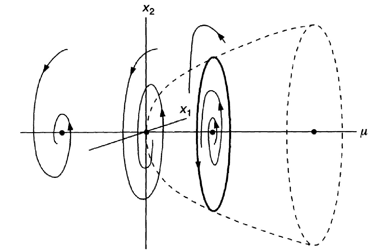
Figure 5.9
Hopf bifurcation: when \(\mu\) increases, the stable
focus becomes unstable, and a periodic solution called \emph{limit
cycle} appears.
This is an example of a Hopf bifurcation, also known as
Poincar\'{e}-Andronov-Hopf bifurcation. As the parameter is varied,
a stationary point changes its stability and a periodic orbit is created
with the opposite stability (like a pitchfork bifurcation in \(r\)).
If the bifurcating periodic orbit is stable, then this is a
\emph{supercritical Hopf bifurcation} and if it is unstable
this is a \emph{subcritical Hopf bifurcation}. The above canonical
example can also be written with complex numbers. That is, if we define
\(z(t) = x(t) + iy(t)\), then the above system is equivalent to
\[
\frac{d}{dt} z = (\mu + i\omega) z -z|z|^2.
\]
If only the first equation in \eqref{Hopf} in
the radial variable \(r\) is taken, a pitchfork bifurcation
happens at \(\mu=0\). This connection (at least qualitatitively)
between Hopf bifurcation (for two variables) and pitchfork bifurcation
(in radial like variable) is true in general.
Example 5.5 (Brusselator model for autocatalytic reaction)
Consider the system of ODEs
\[
\dot{x} = a-(b+1)x+x^2y,\qquad
\dot{y} = bx-x^2y,
\]
where \(a\) and \(b\) are two positive parameters.
The unique steady state is \((a,b/a)\) with the Jacobian
\[
J = \begin{pmatrix} b-1& a^2 \cr -b & -a^2\end{pmatrix}.
\]
Since the determinant of \(J\) is \(a^2\), the only possible bifurcation
Hopf bifurcation, which occurs only when the trace is zero. That
is when \(b^*=1+a^2\). For \( b < b^*\), the steady state \((a,b/a)\) is stable; for \( b>b^*\), it is unstable and a new periodic solution
(a limit cycle) appears.
Example 5.6
We considered in Example 4.3 the following model
\[
\dot{x} = -x+ay+x^2y,\qquad \dot{y} = b-ay-x^2y
\]
for glycolysis oscillation with \(b=1/2\) and \(a>0\). For general \(b\), the only stationary point is
\[
x^* = b,\qquad y^* = \frac{b}{a+b^2}.
\]
We can find the conditions for possible bifurcations. From the Jacobian matrix
\[
J(x,y) = \begin{pmatrix}
-1+2xy & a+x^2\cr -2xy & -a-x^2,
\end{pmatrix}
\]
we have
\[
J(x^*,y^*) = \begin{pmatrix}
\frac{b^2-a}{b^2+a} & a+b^2 \cr -\frac{2b^2}{a+b^2} & -a-b^2
\end{pmatrix}
\]
Since \(\mbox{det} J(x^*,y^*)=a+b^2>0\), the only possible bifurcation is
the real parts of the complex eigenvalues pass zero (real eigenvalues can not
pass zero, which leads to zero determinant), or Hopf bifurcation. This happens
when the trace of \(J(x^*,y^*)\) is zero, that is,
\[
\mbox{tr} J(x^*,y^*) = \frac{b^2-a-a^2-2ab^2-b^4}{a+b^2}.
\]
If \(\mbox{tr} J(x^*,y^*)<0\), the fixed point \((x^*,y^*)\) is stable; otherwise it is not stable.
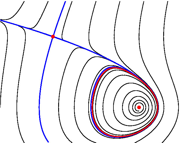
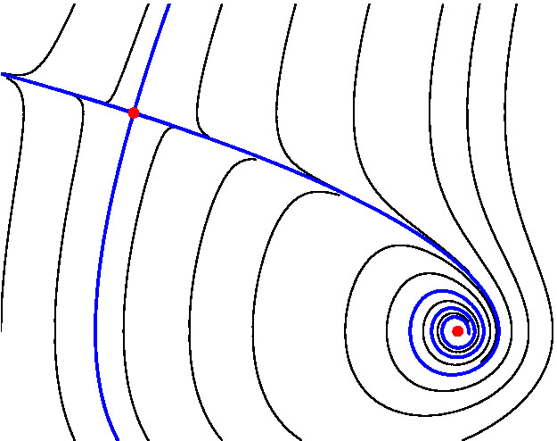
Figure 5.10
The phase portrait of the system \eqref{eq:bifurphase} for \(\mu=1.8\) (left figure)
and \(\mu=2.2\) (right right). As \(\mu\) passes \(2\), the periodic solution (or the limit
cycle) disappear, and the unstable focus at \((\mu-1,-1)\) becomes a stable focus. (Can you
add arrows to indicate the direction of the trajectories, based on the local behaviours
of the stationary points?)
Example 5.7
Consider the
following system
\begin{equation}\label{eq:bifurphase}
\dot{x} = 1-y^2,\qquad \dot{y} = -x-\mu y -y^2,
\end{equation}
for \(\mu \geq 0\).
The fixed points are \((\mu-1,-1) \) and \((-\mu-1,1)\) with the
Jacobian matrix is \(J=\begin{pmatrix} 0 & -2y\cr -1 & -\mu -2y
\end{pmatrix}\).
At the fixed point \((-\mu-1,1)\), \(
J=\begin{pmatrix} 0 & -2 \cr -1 & -\mu-2\end{pmatrix}\). Since
\(\mbox{det} J = -2<0\), the two eigenvalues have opposite signs, and this is always a saddle point. At the fixed point \((\mu-1,-1)\), \( J=\begin{pmatrix} 0 & 2 \cr -1 & -\mu+2 \end{pmatrix} \) and the eigenvalues are the roots of \[ \lambda^2 + (\mu-2)\lambda + 2=0, \] or \(\lambda_\pm=\frac{2-\mu\pm \sqrt{\mu^2-4\mu-4}}{2}\). Since \(\lambda_+\lambda_-=2>0\), the real parts of the eigenvalues
pass zero if and only if \(\mu\) passes 2. At \(\mu=2\),
the two eigenvalues are \(\pm \sqrt{2} i\), this is
a unstable focus becomes a stable focus. When \(\mu\) continues
to increase beyond \(1+2\sqrt{2}\), the discriminant
\(\Delta = \mu^2-4\mu-4\) becomes positive, and the two eigenvalues
are both real and negative. Therefore, the stable
focus becomes a stable node, as shown in Figure 5.11.
Figure 5.11
The global bifurcation at about \(\mu^*=1.63\),
where there is a homoclinic orbit at \((-\mu-1,1)\).
There is actually another bifurcation at about \(
\mu^*=1.63\), with a homoclinic orbit at the fixed point
\((-\mu-1,1)\): the unstable manifold \(W^u\) coincides with
the stable manifold \(W^s\) through this fixed point. This
kind of \emph{global bifurcation} is much more difficult to study,
where the critical parameter \(\mu^*\) can not be determined
as the local bifurcation in the previous few examples.
You can move the slider to choose different values of \(\mu\)
for the system \(\dot{x} =1-y^2,\dot{y}=-x-\mu y - y^2\)
considered in Example 5.7.