
We have seen that if \(\mathrm{Re} \lambda_i < 0\) for all eigenvalues \(\lambda_i\) of \(A\), solutions of linear system \(\dot{x}=A x\) converge to the origin. In fact, if \(A\) can be diagonised with the eigenpairs \((\lambda_i,e_i)\), then the solution can be written as \[ x(t)=\sum_{i=1}^n c_i e^{\lambda_i t} e_i, \] while the prefactor \(e^{\lambda_i t}\) goes to zero as \(t\) goes to infinity. Is this true of the corresponding nonlinear system near the stationary point, when the solution can not be obtained in explicit form? This is part of a much more general question about stability of stationary points, so first let us introduce some definitions. The main questions to be answered in this subsection are: (1) How do stability results for linear systems carry over to nonlinear systems locally? (2) How about the boundedness or stability of solutions for \(\dot{x}=f(x), x \in \mathbb{R}^n\).
A stationary point \(x^*\) of an autonomous system \(\dot{x}=f(x)\) is asymptotically stable iff there exists an open neighbourhood \(U\) of \(x^*\) such that \(\varphi_t(x_0) \to x^*\) as \(t \to \infty\) for all \(x_0 \in U\).
If all eigenvalues \(\lambda_i\) are negative, then the solution starting at any \(x_0\) converges to the origin. If \(A=\mbox{diag}(\lambda_1,\lambda_2,\cdots,\lambda_n)\) is diagonal, this asymptotical stability can also be shown alternatively by considering the (squared) distance \(V(x)=| x|^2\) between the solution \(x(t)\) and the origin. Since \[ \frac{d}{dt} V(x)=2 x\cdot \dot{x}=2 \sum_{i=1}^n \lambda_i x_i^2\leq 0, \] the square distance \(|x(t)|^2\) is strictly decreasing, until \(x(t)\) reaches the origin. This means that \(V(x(t))=|x(t)|^2\) converges to zero .
This means that if a solution starts sufficiently close to \(x^*\), itsfisolution eventually becomes arbitrary close to \(x^*\). But it does not implyfithe solution stays within \(U\) for all \(t>0\).
A stationary pointfi\(x^*\) of an autonomous ODE is Lyapunov stable iff for every openfineighbourhood \(U\) of \(x^*\) there exists an open neighbourhood \(W \subset U\) such that \(x_0 \in W\) implies \(\varphi_t(x_0) \in U\) for all \(t \ge 0\).
In other words solutions stay close to \(x^*\) if they start closefienough to \(x^*\). Note that Lyapunov stability does not imply asymptoticfistability (think of a linear centre). We have been thinking about linearisation,fiwhich motivates our final definition.
A stationary point \(x^*\) of anfiautonomous ODE is linearly stable iff the real parts of everyfieigenvalue of \({D}f(x^*)\) is negative.
For linear systemsfi\(\dot{x}=Ax\), if the eigenvalues of \(A\) have negative real parts thenfi\(|x(t)|\to 0\) as \(t \to \infty\), i.e. solutions are asymptotically stablefi(we have shown this in the special case of distinct eigenvalues). We will take a geometric view of stability (see the textbook byalues). Meiss for a more analytic treatment). The geometric approach is via motivatingalues). example for showing solutions are bounded (often an important first step inalues). The proof of the lemma uses some results from calculus. First recall the chain rule for the derivative of a function of a function. In one dimension \[ \frac{\mathrm{d}}{\mathrm{d} t}V(x(t)) =\frac{\mathrm{d} V(x(t))}{\mathrm{d} x}\frac{\mathrm{d} x(t)} {\mathrm{d} t} \] and in higher dimensions (\(x(t)\in\mathbb{R}^n\)) \[ \frac{\mathrm{d}}{\mathrm{d} t}V(x(t))=\nabla V(x(t)) \cdot \frac{\mathrm{d} x(t)}{\mathrm{d} t} =\nabla V(x)\cdot \dot{x}. \] So if \(x\) satisfies the differential equation \(\dot x=f(x)\) then \[ \frac{\mathrm{d}}{\mathrm{d} t}V(x(t))=\nabla V(x) \cdot f(x) . \]
Bounding Lemma Consider \(\dot{x}=f(x)\), \(x \in \mathbb{R}^n\), \(f\) smooth. Suppose there exists a compact set \(U \subset \mathbb{R}^n\), \(\epsilon >0\) and a continuously differentiable function \(V:U\to \mathbb{R}\) such that
then for all \(x_0 \in \mathbb{R}^n\) there exists \(t_0> 0 \) such that \(\varphi_t(x_0) \in S_{c_0}\) for all \(t \ge t_0.\)
Proof We first show that \(x(t)\) enters \(S_{c_0}\) at some time,
even initially \(x_0\) is not in \(S_{c_0}\). If \(x_0 \notin S_{c_0}\), then \(\dot{V} < - \varepsilon\) and \(V(x_0)>c_0\), so \begin{equation*}
V(\varphi_t(x_0)) < V(x_0) - \varepsilon t, \end{equation*} and so there
exists \(t_0 < \frac{V(x_0) - c_0}{\varepsilon}\) such that
\begin{equation*} V(\varphi_{t_0}(x_0))=c_0,
\qquad \text{ i.e. } \varphi_{t_0}(x_0) \in S_{c_0}.
\end{equation*}
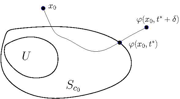
Once \(x(t)\) is in \(S_{c_0}\), we show that it stays in \(S_{c_0}\). To make this argument formally, suppose \(\varphi_{t^*}(x_0) \in \partial S_{c_0}\) and for \(\delta>0\) sufficiently small \(\varphi_t(x_0) \notin S_{c_0}\), for any \(t \in (t^*,t^*+\delta)\) (see Figure 3.14). Then \( V(\varphi_{t^*+\delta}(x_0))>c_0 = V(\varphi_{t^*}(x_0)) \) and \( \dot{V}(\varphi_t(x_0))<-\epsilon \) for any \( t \in (t^*,t^*+\delta) \). Then \[ 0< V(\varphi_{t^*+\delta}(x_0)) - V(\varphi_{t^*}(x_0))=\int_{t^*}^{t^*+\delta} \frac{\mathrm{d}}{\mathrm{d} t} V(\varphi_t(x_0))\mathrm{d} t < \int_{t^*}^{t^*+\delta} (-\epsilon)\mathrm{d} t=-\delta \epsilon. \] So we get a contradiction.
The same basic idea works for stationary points, leading to the so called Lyapunov functions.
A function \(V:U\to \mathbb{R}\) is called a Lyapunov function on \(U \subseteq \mathbb{R}^n\) iff it is continuously differentiable, \(V(x) \ge 0\) on \(U\) and \(\dot{V}\le 0\) on \(U\).
Lyapunov's Stability Theorem Suppose \(x^* \in \mathbb{R}^n\) is a)stationary point of \(\dot{x}=f(x)\) with \(f\) smooth. Let \(U\) be an open neighbourhood of \(x^*\) and suppose there exists a Lyapunov function \(V:U \to \mathbb{R}\) such that \(V(x) >0\) on \(U \setminus \{x^*\}\) and \(V(x^*)=0\). Then \(x^*\) is Lyapunov stable. If in addition \(\dot V<0\) in \(U \setminus \{x^*\}\) then \(x^*\) is asymptotically stable.
Proof. Choose \(\varepsilon>0\) small enough so that \(\{ x \mid |x-x^*|)\le \varepsilon \}\) lies entirely in \(U\), and let \(\displaystyle c_0= \min_{|x-x^*| = \varepsilon} V(x)\) which exists as \(|x-x^*|=\varepsilon\) is compact (closed and bounded), and \(c_0>0\) as \(x^* \notin \{ x \mid | x-x^*| =\varepsilon\}\). Let \(\mathcal{B}_\varepsilon(x^*) = \{ x \mid |x-x^*| <\varepsilon \}\). Now \(V\) is continuous, and \(V(x^*)=0\), so there exists \(\delta>0\) such that for all \(x \in \mathcal{B}_\delta(x^*), V(x) <\frac{1}{2} c_0.\) Consider \(x_0 \in \mathcal{B}_\delta (x^*).\) Since \(\dot{V} \le 0\) in \(U\), \(V(\varphi_t(x_0)) \le V(x_0) < \frac{1}{2} c_0\) for all \(t\) such that \(\varphi_t(x_0) \in U\), and hence \(V(\varphi_t(x_0))<\frac{1}{2}c_0 < c_0\), the minimum on \(|x-x^*|=\varepsilon\). Hence \(\varphi_t(x_0)\in \mathcal{B}_\varepsilon(x^*)\) for all \(t>0\).

Suppose in addition that \(\dot{V}<0\) if \(x\in U \backslash \{x^*\}\), (note that \(\dot{V}(x^*)=0\) since \(x^*\) is stationary). Then if \(x_0 \in \mathcal{B}_\delta(x^*)\) as before, \(V(\varphi_t(x_0))\) is strictlyfidecreasing and hence tends to a limit \(\bar{V}=\lim_{t\to\infty} V(\varphi_t(x_0))\). At the limit \(\dot{V}=0\) hence the limit must be \(x^*\).
In many practical examples, the stationary point \(x^*\) can still be asymptotic stable, when the condition \(\dot{V} < 0\) in \(U\subset \{x^*\}\) in Lyapunov's Stability Theorem can be relaxed to \(\dot{V} \leq 0\), provided that \(x^*\) is the only fixed point.
Theorem (LaSalle's Invariance Principle) Suppose that \(V: U\subset \mathbb{R}^n \to \mathbb{R}\) is a Lyapunov function for the system \(\dot{x}=f(x)\). If the set \(\{x\in U \mid \dot{V}(x)=0\}\) contains only one fixed point \(x^*\), then \(x^*\) is asymptotically stable.