The previous result shows that if \(\mbox{Re} (\lambda)<0\) and the eigenvalues are distinct, then a linearly stable fixed point is locally stable when nonlinear terms are added back in. This is an example of a range of persistence results for behaviour.
Figre 3.16 Invariant manifolds \(W^s\) and \(W^u\) for the linearised system and full nonlinear system
in Example 3.10.
Example 3.10
The linearised system of the full nonlinear system
\[
\dot{x} = -x,\quad \dot{y} = y+x^2
\]
is \(\dot{x}=-x, \dot{y}=y\), with two eigenvalues \(\pm 1\). The phase portrait for this
saddle system should be well known now, but there are two special straight lines deserving
more attention: the \(x\)-axis and and the \(y\)-axis. If the initial condition \((x_0,y_0)\)
is on the \(x\)-axis (that is \(y_0=0\)), then the solution \((x(t),y(t))\) converges to the origin,
as time \(t\) goes to infinity. This linear space is called the stable manifold,
denoted as \(E^s\). Although the solution with initial condition away from the
\(x\)-axis goes not infinity, as time \(t\) goes to positive infinity, initial condition
\((x_0,y_0)\) resides on the \(y\)-axis has the special property that its solution
converges to the origin as time \(t\) goes to negative infinity. The \(y\)-axis
is called unstable manifold (which is the stable manifold when time is reversed),
denoted as \(E^u\).
Back to the nonlinear system, the correponding phase portrait is deformed from
that of the linearised system. There are also special curves, the stable manifold \(W^s\)
and the unstable manifodl \(W^u\), whose solution converges to the origin, as time \(t\)
goes to positive infinity and negative infinity, respectively. In general, \(W^s\) (or \(W^u\))
is no longer straight line, but it is tangent to \(E^s\) (or \(E^u\)) at the origin.
In fact, in this example, we can find the equations for \(W^s\) and \(W^u\). Obviously, \(W^u\)
is the \(y\)-axis: if \(x_0=0\), then the ODE \(\dot{x}=-x\) implies \(x(t) = x_0e^{-t}\equiv 0\),
and \(y(t) = y_0e^t \to 0\) as \(t \to -\infty\). The stable manifold is \(W^s = \{
(x,y) \mid y=-x^2/3\}\). If \((x_0,y_0)\) is on \(W^s\), that is \(y_0=-x_0^2/3\), then
\(x(t) = x_0e^{-t}\) and \(y\) satisfies the linear ODE
\[
\dot{y} = y + x_0^2e^{-2t}.
\]
From the fact that \(\frac{\mathrm{d} }{\mathrm{d} t}\big( e^{-t}y\big) =
e^{-t} (\dot{y}-y) = x_0^2e^{-3t}\), we get
\[
e^{-t}y(t) = y_0 + \int_0^t x_0^2e^{-3\tau}\mathrm{d} \tau = y_0 + \frac{x_0^2}{3}\big(1-e^{-3t}\big)
=\left(y_0+\frac{x_0^2}{3}\right)-
\frac{x_0^2}{3}e^{-3t}
=- \frac{x_0^2}{3}e^{-3t}.
\]
Since the solution \((x,y) = \left(x_0e^{-t},-\frac{x_0^2}{3}e^{-2t}\right)\)
stays on \(W^s\) and converges to the origin (as \(t\) goes to positive infinity),
\(W^s\) is a stable manifold.
Here the word manifold is used for a smooth geometric curve or
surface: if the manifold
is one dimension, it is a smooth curve (inluding straight lines);
if the manifold is two dimension, it is a smooth surface (including planes).
But normally we do not know the dimension of the curve or the surface in
advance, so it is better to use the generic name manifold
instead of the more common curve or surface.
This above relationship between full system and its linearised system is summarised
in the following theorem, provided that none of the eigenvalue has zero real part.
Theorem(Stable Manifold Theorem)
Suppose \(\dot{x}= Ax+O(x^2)\) and \(A\) has no eigenvalues with \(\Re (\lambda)=0\) (\(x=0\) is called a hyperbolic stationary point in this case). Then after a change of coordinates the system is
\begin{align*}
\dot{x}_1 = A^+ x_1 + O(|x|^2) ,\qquad
\dot{x}_2 = A^- x_2 + O(|x|^2)
\end{align*}
where \(A^+\) has \(\Re(\lambda)>0, A^-\) has \(\Re(\lambda)<0\). Moreover there are invariant manifolds \(W^u\) and \(W^s\) with \begin{equation*} W^u=\left\{ x \in U \mid \varphi_t(x) \to 0 \text{ as } t \to -\infty \right\} \end{equation*} and \begin{equation*} W^s=\left\{ x \in U \mid \varphi_t(x) \to 0 \text{ as } t \to \infty \right\}. \end{equation*} which are of of the same dimension as \(x_1\) (resp. \(x_2\)) and tangential to \(x_2=0\) (resp. \(x_1=0\)) at the origin.
This implies the persistence of saddle structure near a stationary point
when the nonlinear terms are added back into the linearisation. The correponding changes
in the phase portraits or the deformation of the stable/unstable manifolds are
best discribed using language from topology (think about the deformation
of a coffee mug into a donut). The persistence between structure are called topologically
conjugate or topologically equivalent, but we will omit this complicated topological
language and keep a mental picture instead, as in the following theorem.
Hartman--Grobmann Theorem
If \(\dot{x}=Ax+O(x^2)\) and \(A\) has no eigenvalue with zero real part, then the behaviour
near the neighbourhood of the origin is topologically equivalent to the linear system \(\dot{x}=Ax\).
Example 3.11
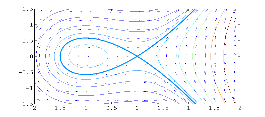
Now consider the system \(\dot{x} = y,\dot{y}=x^2+x\) and its
linearised system \(\dot{x}=y,\dot{y}=x\). The trajectories, governed by
\(\frac{\mathrm{d} y}{\mathrm{d} x}
=\frac{x^2+x}{y}\)(which is separable), are given by
\(\dfrac{x^3}{3}+\dfrac{x^2-y^2}{2}=C\). The stable manifold \(W^s\) concides
with the unstable manifold \(W^u\), and is \(\dfrac{x^3}{3}+\dfrac{x^2-y^2}{2}=0\).
Figure 3.17
The phase portrait for \(\dot{x}=y,\dot{y}=x^2+x\) in Example 3.11.
If \(A\) has eigenvalue with zero real part, then the situation is much more complicated, as we can see from the following two examples.
Example 3.12 Consider the system \(\dot{x} =x, \dot{y}=y^2\), which you can solve the individual equations separately (they are de-coupled from each other). The lienarized
system (near the origin) \(\dot{x} = x, \dot{y}=0\) has only horizontal phase curves.
For a related system \(\dot{x}=y^2,\dot{y}=x\) (you can also solve this explicitly).
If there is zero eigenvalue in the linearised system,
their local behaviours of the full nonlinear system near the fixed point
are different, as we can see from Figure 3.18 and 3.19.
Figure 3.18
Phase portraits for the system
\(\dot{x}=x, \dot{y}=y^2\) with zero eigenvalues at the origin.
Figure 3.19
Phase portraits for the system
\(\dot{x}=y^2, \dot{y}=x\) with zero eigenvalues at the origin.
Exercise
Find the solution to the system
\[
\dot{x} = x,\qquad \dot{y} = y^2
\]
and
\[
\dot{x} = y^2,\quad \dot{y}= x
\]
whose phase portraits are given in Figure 3.18 and 3.19.
Click on the plane to see how the solutions of the system
\[
\dot{x} = x,\qquad
\dot{y} = y^2
\]
differ from its linearised system \(\dot{x}=x,\dot{y}=0\)
(where everything moves away from the \(y\)-axis horizontally), especially when \(|y|\) is not small.
On the other hand, if \(y\) is small, the behaviours of the two systems do look similar.
The situation is even worse for the system \(\dot{x} = f(x)\) if \(f(x) = O(|x|^2)\), because the linearised
system \(\dot{x}=0\) does not tell anything about the behaviour of the system
near the origin. You can see two examples in
Figure 3.20. Information can still be obtained in certain cases,
by looking at the trajectories, or by transforming into polar coordinates.
Figure 3.20
Phase portraits for systems with zero linear parts at the
origin: Left:
\(\dot{x}=-xy, \dot{y}=x^2+y^2\); Right: \(\dot{x}=x^2,\dot{y}=y(2x-y)\).
Example 3.13 Consider the system
\(
\dot{x} = -xy, \dot{y} = x^2+y^2,
\)
whose phase portrait is given in Figure 3.20(left figure). The trajectory,
governed by the ODE \(\frac{\mathrm{d} y}{\mathrm{d} x}
= -\frac{x^2+y^2}{xy}\) is homogeneous. By the change
of variable \(y=zx\), the ODE becomes \(\frac{\mathrm{d} z}{\mathrm{d} x}
= -\frac{2z^2+1}{z}x\), which is
separable. The solution is given by \(x^4(2z^2+1)=C\) and the
trajectories are given by \(2x^2y^2+x^4=C\).