Visualising the Wishart Distribution
This semester, I have been teaching Multivariate Statistics, and one isse that comes up is how to think about the Wishart distribution, which generalises the \(\chi^2 \) distribution. This has probability density function
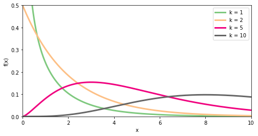
$$ f_{\chi^2_k}(x) = \frac{1}{2\,\Gamma\!\left(\frac{k}{2}\right)} \left(\frac{x}{2}\right)^{\frac{k}{2}-1} {\rm e}^{-\frac{x}{2}} . $$
To visualise this at different degrees of freedom \(k \), we use the following Python code.
%matplotlib inline
import numpy as np
import scipy.stats as st
import matplotlib.pyplot as plt
from mpl_toolkits.mplot3d import Axes3D
x = np.linspace(0, 10, 1000)
plt.figure(figsize=(8,4))
colors = plt.cm.Accent(np.linspace(0,1,4))
i=0
for k in (1,2,5,10):
    c = st.chi2.pdf(x, k);
    plt.plot(x,c, label='k = ' + str(k), color=colors[i],linewidth=3)
    i += 1
plt.xlim((0,10))
plt.ylim((0,0.5))
plt.xlabel('x')
plt.ylabel('f(x)')
plt.legend()
The Wishart emerges when we make \(k \) observations each with \(p \) variables; the sampling distribution for the covariance matrix of these data if the population is multivariate normal is Wishart and has probability density function
$$ f_{\mathcal{W}_p(k,\boldsymbol{\Sigma})}(\boldsymbol{V}) = \frac{\mathrm{det}(\boldsymbol{V})^{\frac{k - p - 1}{2}}}{2^{ \frac{k p}{2} } \mathrm{det}(\boldsymbol{\Sigma})^\frac{k}{2} \Gamma_p\!\left(\frac{k}{2} \right)} \exp\left( -\frac12 \mathrm{Tr}(\boldsymbol{\Sigma}^{-1} \boldsymbol{V}) \right) . $$
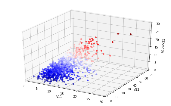
In general, this cannot be visualised, but for the \(p=2 \) case, one option is to pick random numbers from this distribution and then produce a three-dimensional scatter plot of these. The code and results below show that this can be seen as behaving somewhat like the chi-squared distribution that it generalises as the degrees of freedom \(k \) are increased.
x=np.zeros(n)
y=np.zeros(n)
z=np.zeros(n)
for i in range(0,n):
    M=st.wishart.rvs(2,scale=Sig1,size=1)
    x[i]=M[0][0]
    y[i]=M[1][1]
    z[i]=M[1][0]
fig = plt.figure(figsize=(8,5))
ax = fig.add_subplot(111, projection='3d')
ax.scatter3D(x,y,z, marker='o', c=z, cmap='seismic')
ax.set_xlabel('V11')
ax.set_ylabel('V22')
ax.set_zlabel('V12=V21')
ax.set_xlim((0,30))
ax.set_ylim((0,70))
ax.set_zlim((0,30))
plt.tight_layout()

x=np.zeros(n)
y=np.zeros(n)
z=np.zeros(n)
for i in range(0,n):
    M=st.wishart.rvs(5,scale=Sig1,size=1)
    x[i]=M[0][0]
    y[i]=M[1][1]
    z[i]=M[1][0]
fig = plt.figure(figsize=(8,5))
ax = fig.add_subplot(111, projection='3d')
ax.scatter3D(x,y,z, marker='o', c=z, cmap='seismic')
ax.set_xlabel('V11')
ax.set_ylabel('V22')
ax.set_zlabel('V12=V21')
ax.set_xlim((0,30))
ax.set_ylim((0,70))
ax.set_zlim((0,30))
plt.tight_layout()
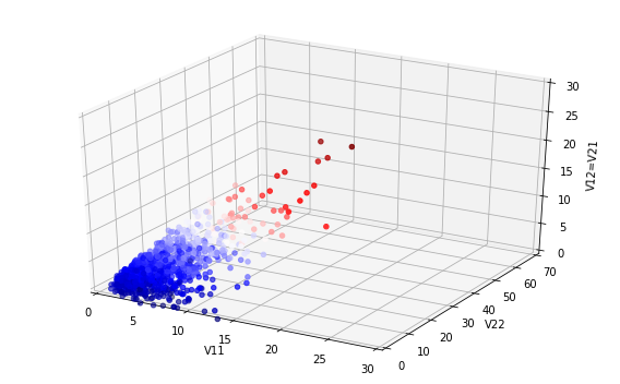
x=np.zeros(n)
y=np.zeros(n)
z=np.zeros(n)
for i in range(0,n):
    M=st.wishart.rvs(10,scale=Sig1,size=1)
    x[i]=M[0][0]
    y[i]=M[1][1]
    z[i]=M[1][0]
fig = plt.figure(figsize=(8,5))
ax = fig.add_subplot(111, projection='3d')
ax.scatter3D(x,y,z, marker='o', c=z, cmap='seismic')
ax.set_xlabel('V11')
ax.set_ylabel('V22')
ax.set_zlabel('V12=V21')
ax.set_xlim((0,30))
ax.set_ylim((0,70))
ax.set_zlim((0,30))
plt.tight_layout()