Time-Lapse Hyperspectral Radiance Images of Natural Scenes 2015
1. Scenes
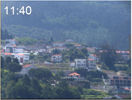
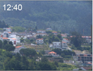
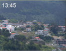
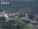
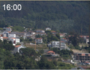
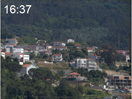
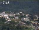
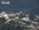
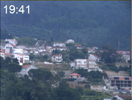
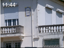
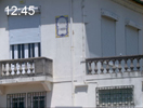
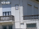
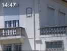
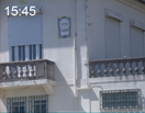
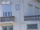
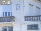
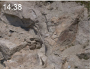
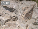
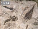
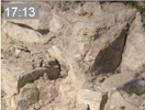
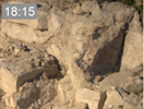
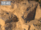
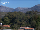
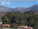
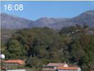
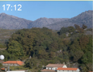
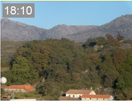
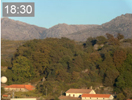
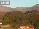
These sequences of hyperspectral radiance images have been taken from a study by Foster, Amano, and Nascimento (2016) of scenes undergoing natural illumination changes. In each scene, hyperspectral images were acquired at about 1-hour intervals. Thumbnail RGB images from the sequences are shown below with times and dates of acquisition.
Each hyperspectral radiance image along with a full-size rendered RGB image and an information document can be downloaded as a zipped file (< 340 MB) by clicking on the "HSI" link beneath each thumbnail. The information document can be viewed separately as a PDF file by clicking on the adjacent "Information" link. The information document is common to all the images in a time-lapse sequence.
Details of image acquisition, image processing, and contents of each file are given further down this page.
These data are for personal use only. If you use the hyperspectral radiance images or the colour images rendered from them in published work, please cite the source publication: Foster, D.H., Amano, K., & Nascimento, S.M.C. (2016). Time-lapse ratios of cone excitations in natural scenes. Vision Research, 120, 45-60.doi.org/10.1016/j.visres.2015.03.012
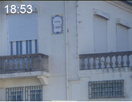
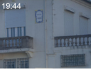
Nogueiró scene (acquired 9 June 2003)
 |
 |
 |
 |
 |
| HSI | Information | HSI | Information | HSI | Information | HSI | Information | HSI | Information |
 |
 |
 |
 |
|
| HSI | Information | HSI | Information | HSI | Information | HSI | Information |
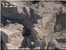
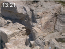
Gualtar scene (acquired 6 June 2003)
 |
 |
 |
 |
 |
| HSI | Information | HSI | Information | HSI | Information | HSI | Information | HSI | Information |
 |
 |
 |
 |
|
| HSI | Information | HSI | Information | HSI | Information | HSI | Information |
Sete Fontes scene (acquired 6 October 2003)
 |
 |
 |
 |
 |
| HSI | Information | HSI | Information | HSI | Information | HSI | Information | HSI | Information |
 |
 |
 |
||
| HSI | Information | HSI | Information | HSI | Information |
Levada scene (acquired 8 October 2003)
 |
 |
 |
 |
 |
| HSI | Information | HSI | Information | HSI | Information | HSI | Information | HSI | Information |
 |
 |
|||
| HSI | Information | HSI | Information |
2. HSI files
Each zipped HSI file contains a
hyperspectral
radiance image file in Matlab MAT-file format, labelled by
time,
e.g. the image of the Nogueiró scene at 11:40 is called
"nogueiro_1140.mat". Each
hyperspectral image has
dimensions 1024 × 1344 × 33 and represents a set of 33
greyscale
images of size 1344 (H) ×
1024 (V) pixels sampled at wavelengths 400, 410, ..., 720 nm, with each
pixel value
representing spectral radiance in W m−2 sr−1
nm−1.
3. Imaging system
The custom-built system comprised a low-noise Peltier-cooled digital camera with CCD sensor (Hamamatsu, model C4742-95-12ER, Hamamatsu Photonics K. K., Japan) and a fast liquid-crystal tunable filter (VariSpec, model VS-VIS2-10-HC-35-SQ, Cambridge Research & Instrumentation, Inc., MA) mounted in front of the lens, together with an infrared blocking filter. The camera provided an effective image size of 1344 × 1024 pixels. The focal length was set typically to 75 mm and aperture to f/16 or f/22 to achieve a large depth of focus. The zoom was set to maximum.
The system line-spread function was close to Gaussian with a standard deviation of approximately 1.3 pixels at 550 nm. The intensity response at each pixel, recorded with 12-bit precision, was linear over the entire dynamic range. The wavelength range of the tunable filter was 400–720 nm. Its bandwidth (FWHM) was 7 nm at 400 nm, 10 nm at 550 nm, and 16 nm at 720 nm. Its tuning accuracy was < 1 nm over 400–660 nm and < 2 nm over 670–720 nm. Errors in peak spectral radiance recorded by the whole system at 436 nm and 546 nm were less than 1 nm at the centre and edges of the imaging field. Root-mean square errors in the recovery of radiance spectra were < 2%, based on measurements of the recovery of spectral reflectance factors of colored samples.
4. Image acqusition
At each scene, the camera system was adjusted for position, viewing direction, focus, and aperture, all of which were then fixed. A small neutral (Munsell N7) flat surface was embedded in the scene to provide a spectral reference and its position and orientation adjusted in relation to the field of view. A small neutral (Munsell N7) glass or plastic sphere was also embedded in all but one scene to help quantify the effects of changing illumination geometry. Around the time of image acquisition, a horizontally oriented barium sulphate plug was introduced to enable estimates to be made of the illumination under direct sunlight and in the shade. The reflected spectrum was recorded with a telespectroradiometer (SpectraColorimeter, PR-650, Photo Research Inc., Chatsworth, CA), whose calibration was traceable to the National Physical Laboratory. The angular subtense of each scene at the camera was approximately 6.9 × 5.3 degrees.
Each time-lapse sequence of hyperspectral images was obtained by making acquisitions at intervals of about one hour, sufficiently long to reveal changes in the distribution of illumination, although with some scenes acquisitions were made more frequently towards the end of the day. Each acquisition, which took a few minutes, comprised three steps. First, the camera exposure time required at each wavelength was determined by an automatic calibration routine that ensured the maximum sensor-element output was within 86%–90% of its saturated value. Second, with exposure times defined, wavelength sequences of raw grayscale images were recorded over the range 400–720 nm at 10-nm intervals. The recording was repeated one or more times within each acquisition period to enable the signal-to-noise ratio (SNR) to be improved (see Section 5). Third, the spectral radiance of the light reflected from the reference surface was recorded from the same viewing direction with the telespectroradiometer. Depending on the scene, acquisitions continued to be made over 9–10 hours or until the level of natural light impeded recording.
5. Image processing
The raw grayscale images were first corrected by subtracting estimates of dark noise and stray light derived from earlier calibration measurements. Spatial non-uniformities (mainly off-axis vignetting) were corrected by dividing by an estimate of the flat-field image. Where recordings of wavelength sequences of images had been repeated, the corrected images at each wavelength were registered over replicates by translation to compensate for any small differences in optical image position and then averaged. They were next registered over wavelength by uniform scaling and translation to compensate for any small differences in optical image size with wavelength (chromatic differences of magnification) and any small differences in optical image position. A few wavelength sequences of images were omitted because their SNRs at 400 nm made registration unreliable.
The resulting hyperspectral image was then calibrated spectrally by applying a spatially uniform spectral correction factor such that the spectral radiance at the neutral reference surface in the image matched the spectral radiance recorded with the telespectroradiometer. The calibrated hyperspectral radiance images from each acquisition period were then assembled to make a time-lapse sequence. Finally, the sequence was registered over acquisition times by translation to compensate for residual differences in optical image position. All image registrations were performed to subpixel accuracy with in-house software.
6. Citing
These data are for personal use only. If you use the hyperspectral radiance images or the colour images rendered from them in any published work arising from these data, please cite the source publication: Foster, D.H., Amano, K., & Nascimento, S.M.C. (2016). Time-lapse ratios of cone excitations in natural scenes. Vision Research, 120, 45-60.doi.org/10.1016/j.visres.2015.03.012