Machine learning is the use of data to tune algorithms for making decisions or predictions. Unlike deduction based on reasoning from principles governing the application, machine learning is a “black box” that just adapts via training.
We divide machine learning into three major forms:
Supervised learning
The training data gives examples that include the answer (or label) we expect to get. The goals are to find important effects and/or to predict labels for previously unseen examples.
Unsupervised learning
The data is unlabeled, and the goal is to discover structure and relationships inherent to the data set.
Reinforcement learning
The data is unlabeled, but there are known rules and goals that can be encouraged through penalties and rewards.
We start with supervised learning, which can be subdivided into two major areas:
Classification, in which the algorithm is expected to choose from among a finite set of options.
Regression, in which the algorithm should predict the value of a quantitative variable.
We will now explore some of the ideas we have learned in Semester 1, chapter “The supervised learning problem”. We will use artificial classification problems to illustrate. We aim to build a better understanding of concepts like the hypothesis, generalisation error, and different loss functions. More practically relevant classification problems and algorithms will be discussed in Chapter 5.
4.1 Creating and working with artificial datasets
Before training any machine learning model on real data, it is usually a good idea to test the model under idealized conditions. Like this, any potential issues can be identified more easily and we can let the model undergo sanity checks such as:
What happens if we have only a single data point? What if we have no data at all?
How does the model scale as the number of data points increases?
How does the data dimensionality affect the model performance? etc.
For example, we could test a classifier first on artificially generated data for which labels are explicitly available.
4.2 Sampling multivariate Gaussians
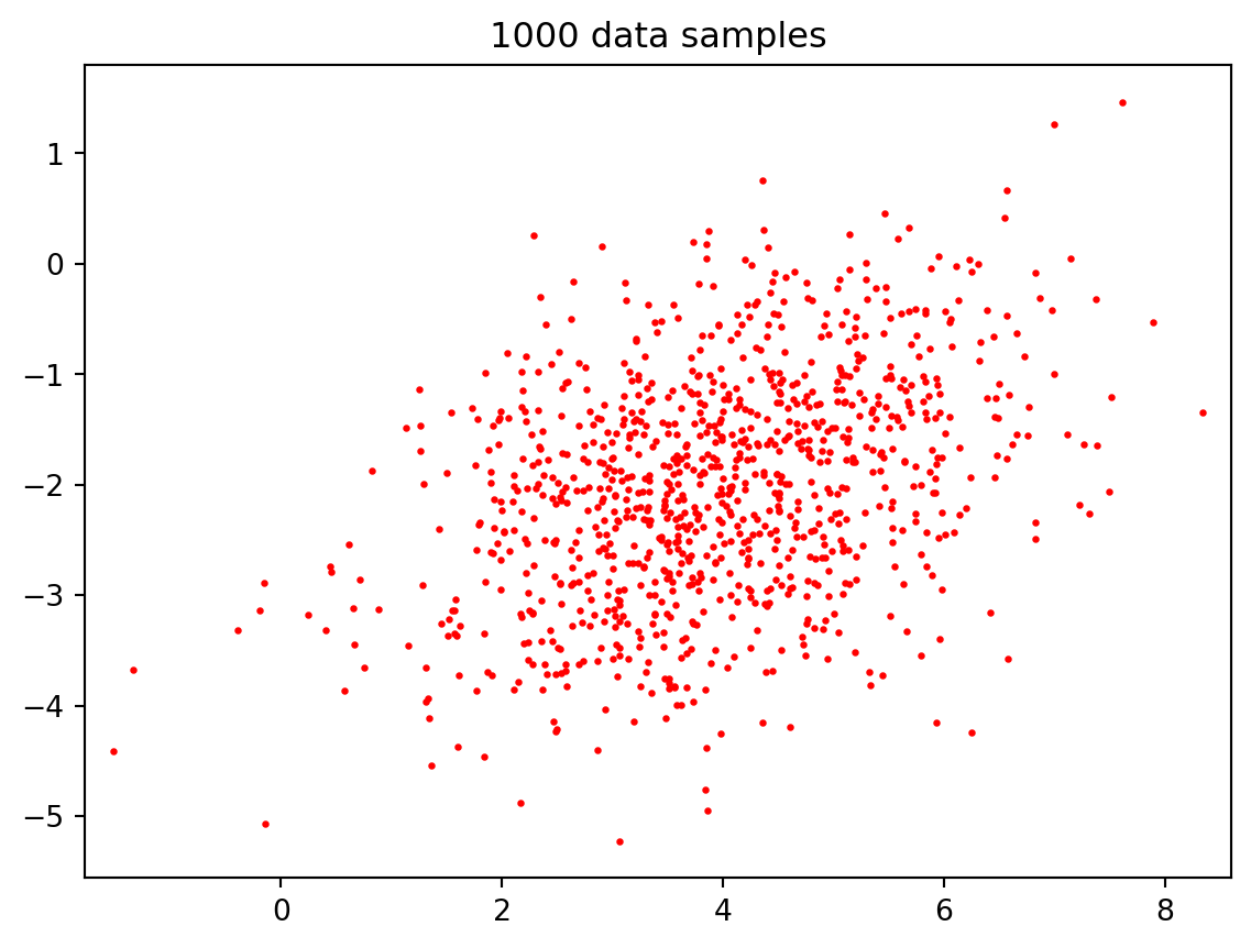
Given a positive definite covariance matrix \(\Sigma\), we can use its Cholesky factorization \(\Sigma = L L^T\) to sample from a multivariate Gaussian distribution as shown below.
import numpy as npimport matplotlib.pyplot as pltfrom numpy.random import default_rngrng = default_rng(0) # good practice for reproducibilitydef gauss_sample(N, c, Sigma):""" returns N samples from a multivariate Gaussian with mean c and covariance matrix Sigma """ m =len(c) L = np.linalg.cholesky(Sigma) z = rng.normal(size=(m, N)) x = c[:,None] + np.dot(L, z)return xN =1000c = np.array([4, -2])Sigma = np.array([[2, 0.5], [0.5, 1]])X = gauss_sample(N, c, Sigma)plt.scatter(X[0,:], X[1,:], s=2, c='r')plt.axis('equal'), plt.title('1000 data samples'); plt.show()# We can use numpy.cov to estimate Sigma from xSigma_est = np.cov(X)print('covariance matrix estimated from data:\n', Sigma_est)
covariance matrix estimated from data:
 [[1.9100027  0.55528846]
 [0.55528846 1.0743857 ]]
Recall the Gaussian density function from part 1 of the course, \[
\pi(x) = (2\pi)^{-m/2} \det(\Sigma)^{-1/2}\exp\left(-\frac{1}{2}\langle x-c, \Sigma^{-1}(x-c)\rangle \right) \qquad (x \in \mathbb{R}^m).
\]
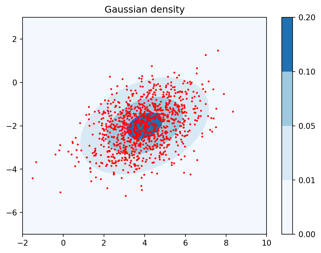
Example 4.1 We can create a contour plot of the Gaussian density in \(m=2\) dimensions as follows.
def gauss_density(x, c, Sigma):""" returns the density of the multivariate Gaussian with mean c and covariance matrix Sigma at x """ m =len(c) norm_const =1/ (np.sqrt((2* np.pi)**m * np.linalg.det(Sigma))) xc = (x - c)[:,None]return norm_const * np.exp(-0.5* np.dot(xc.T, np.linalg.solve(Sigma, xc)))[0,0]# measure runtimefrom time import timest = time()# contour plot of Gaussian density function in 2dx0 = np.linspace(-2, 10, 100)x1 = np.linspace(-7, 3, 100)X0, X1 = np.meshgrid(x0, x1)Z = np.zeros(X0.shape)for i inrange(X0.shape[0]):for j inrange(X0.shape[1]): x = np.array([X0[i, j], X1[i, j]]) Z[i,j] = gauss_density(x, c, Sigma)print("evaluating Z took", time()-st, "seconds")plt.contourf(X0, X1, Z, levels=[0, 0.01, 0.05, 0.1, 0.2], cmap=plt.cm.Blues);plt.colorbar();plt.scatter(X[0,:], X[1,:], s=2, c='r')plt.axis('tight'), plt.title('Gaussian density'); plt.show();
evaluating Z took 0.13178658485412598 seconds
Important
The above coding is very inefficient and can be significantly sped up using vectorisation. See Exercise 4.3.
Note how quickly the density decays away from the mean \(c\). We can numerically check a few facts about that distribution. For example, the area under that surface when integrated over all of \(\mathbb{R}^2\) should be one.
What is the area under the surface whose contour plot we have produced above? To get an approximation, we sum over all of the evaluations of the density in the matrix Z and multiply that by the area of each tiny rectangle produced by meshgrid. This serves as a sanity check that we have got everything right, including the correct normalization constant in the Gaussian probability density formula.
# area of each meshgrid rectangle:rect = (x0[1] - x0[0])*(x1[1] - x1[0]) mass = rect*np.sum(Z)print('Approximate total mass:', mass)
Approximate total mass: 0.9999814403509709
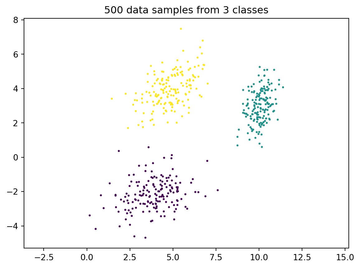
To generate some more interesting data which could arise in a classification setting, we can draw samples from several multivariate Gaussians and superimpose them. (Sklearn has a method sklearn.datasets.make_blobs that does something similar, but it’s easy enough to implement by ourselves and we’ll fully understand what’s going on.)
# list of centers and covariance matrices for each classc_ = { 0: np.array([4, -2]), 1: np.array([10, 3]), 2: np.array([5, 4]) }Sigma_ = { 0: np.array([[2, 0.5], [0.5, 1]]), 1: np.array([[0.3, 0.2], [0.2, 0.8]]), 2: np.array([[1, 0.5], [0.5, 1]]) }def multiple_classes(N, c_, Sigma_):""" returns N samples of 2d data from multiple classes """ nr_classes =len(c_) n0 = N//nr_classes X = np.zeros((2, 0)) y = np.zeros(0)for i inrange(nr_classes):if i == nr_classes-1: n0 = N - (nr_classes-1)*n0 X = np.hstack((X, gauss_sample(n0, c_[i], Sigma_[i]))) y = np.hstack((y, i*np.ones(n0)))# important: always shuffle the order of your data points p = rng.permutation(N) X = X[:,p] y = y[p]return X, yrng = default_rng(1)N =500X, y = multiple_classes(N, c_, Sigma_)plt.scatter(X[0,:], X[1,:], s=2, c=y);plt.title('500 data samples from 3 classes');plt.axis('equal'); plt.show();
Important
We have used NumPy’s permutation method to shuffle the data. Shuffling is extremely important to ensure that we do not ``learn’’ from the order of the data. Scipy also offers a more convenient way to shuffle data with sklearn.utils.shuffle.
4.3 A basic classification task
Imagine that the \(N=500\) data points we have just generated correspond to 500 customers of an online shop, with the two coordinates representing quantities that we can measure for each customer (such as, average time spent on the website versus number of items purchased over the last three years). The marketing department has decided that there are three customer categories and the 500 representative customers have been labelled by hand. In other words, each customber \(x_i\) has been assigned a label \(y_i\in\{0,1,2\}\). The marketing department would like to send personalised emails to customers based on the category they belong to. Can we come up with a machine learning model, based on the training data, to predict the label of a new customer?
This is a very common problem and there are many ways to come up with a classifier, including k-nearest neighbors, decision trees, and neural networks. We will explore some of them later on. But for now, let’s recap some of the theory from the chapter “The supervised learning problem” from part 1 of the course using our 500 example customers.
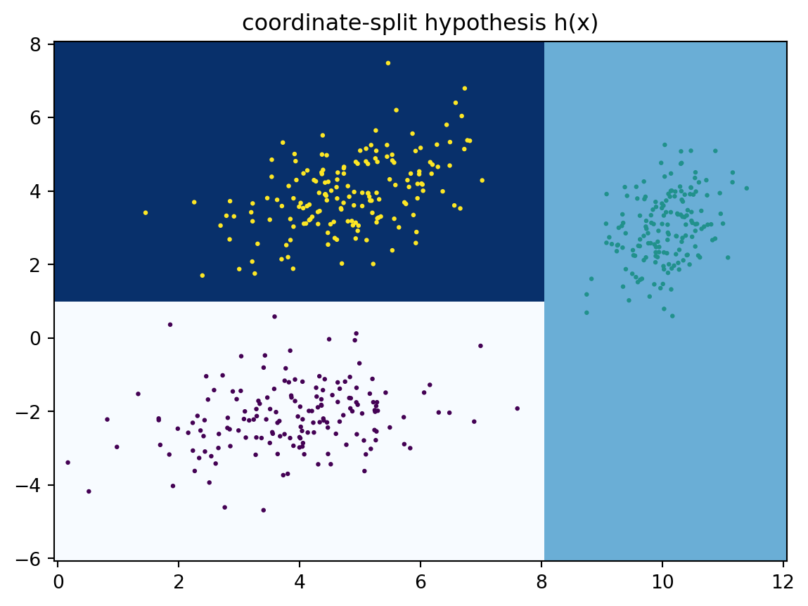
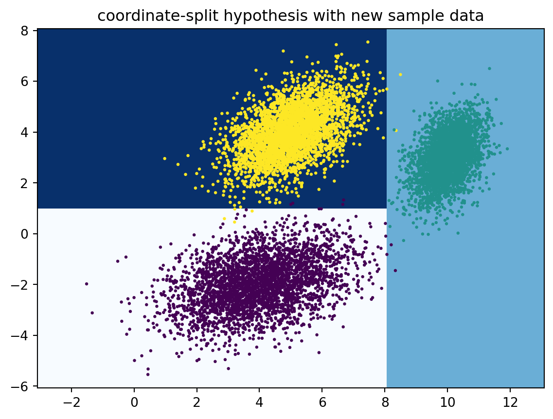
4.3.1 A coordinate-split hypothesis
First of all, we have our input space\(\mathcal{X}=\mathbb R^2\) of data points in two dimensions, and our label space is \(\mathcal{Y}=\{0,1,2\}\). Recall that we defined an hypothesis as a function \(h : \mathcal{X} \to \mathcal{Y}\) that assigns a label \(c(x)\) to a data point (input) \(x\in\mathcal X\). We normally do not know the ‘true hypothesis’ (also called the concept) that generated the data. But as long as the pairs \((x_1,y_1),\ldots,(x_N,y_N)\) are in a functional relation (i.e., such that \(x_i=x_j \Rightarrow y_i=y_j\)), we can retrospectively come up with a ‘perfect’ hypothesis that exactly reproduces the labels. Below is one such hypothesis using a simple coordinate splitting approach.
This coordinate splitting approach is very similar to what is often done in classification with decision trees. We will learn more about that in a following chapter.
Let’s verify that the coordinate-split hypothesis \(h\) indeed explains the labels of our training data perfectly. To this end, we need a loss function \(L:\mathcal{Y}\times \mathcal{Y} \to [0,\infty)\). This loss function \(L\) should be chosen so that \(L(y,y')\) is small if \(y \approx y'\), and large otherwise. In the case of classification, one of the simplest loss functions is the zero-one loss\(L(y, y') = \mathbf{1}[y \neq y']\)\((y, y' \in \mathcal{Y})\). We can then calculate the empirical error\[ \hat{R}(h) := \frac{1}{N}\sum_{n=1}^N L(y_n, h(x_n)), \] which is zero in this case. This means that none of the data points \(x\) has been mislabelled (or, alternatively, all data points have been classified correctly).
loss_01 =lambda y, yp: y != ypdef empirical_err(h, loss, X, y): s =0for n inrange(len(y)): s += loss(y[n], h(X[:,n]))return s/len(y)print('empirical error:', empirical_err(h_coord_split, loss_01, X, y))
empirical error: 0.0
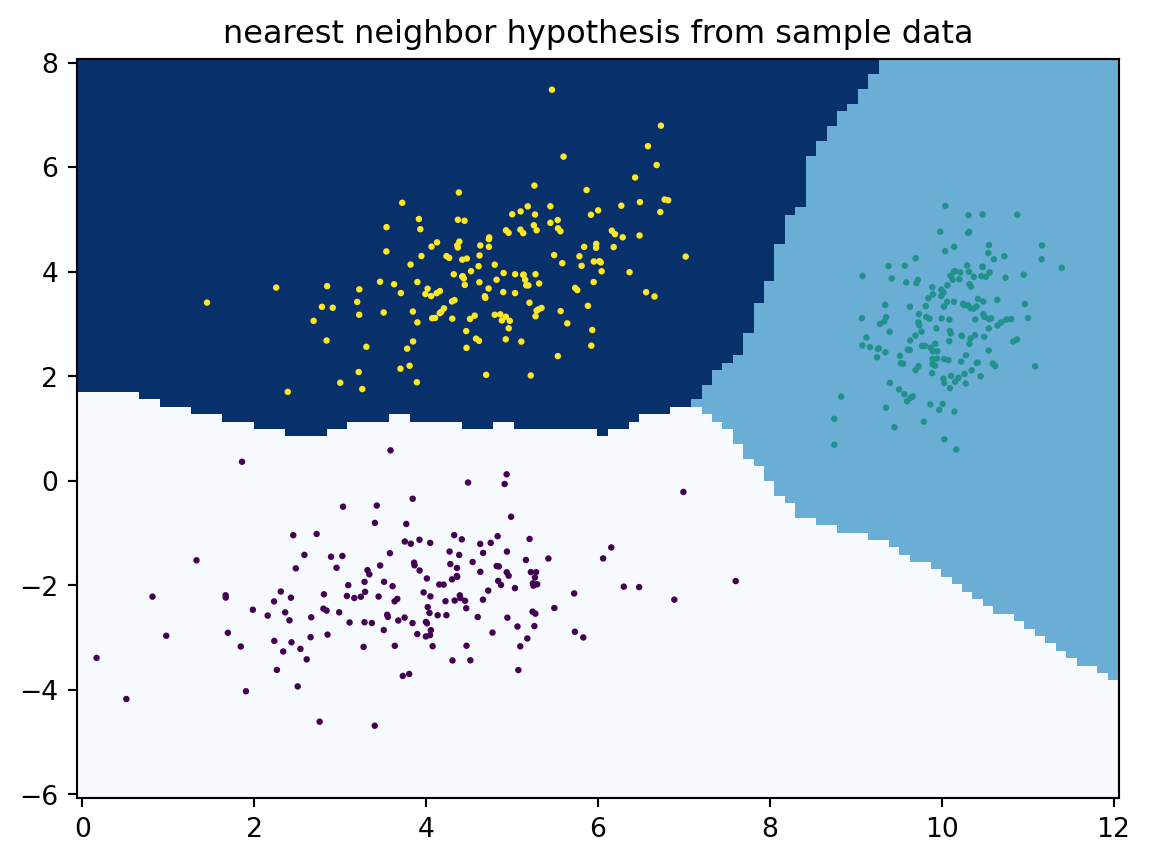
4.3.2 Nearest neighbor hypothesis
Let us give just one example of an alternative model. If we have a distance \(d(x_i,x_j)\) on \(\mathcal{X}\times \mathcal{X}\), we can define a hypothesis using a nearest neighbor approach:
For each \(x\in\mathcal{X}\), find the first \(x_i\) for \(i=1,\ldots,N\) that minimizes \(d(x,x_i).\) Then define \(c(x):=y_i.\)
The below code implements such a nearest neighbor hypothesis using the Euclidean distance. Note how the decision regions become rather complex, and they may even become disconnected in some cases.
Instead of using just a single nearby data point as in the below code, one can take a vote on the \(k\geq 1\) nearest neighbors. More on that in a following chapter.
4.3.3 Classify unseen data
We could use either of the above hypotheses to classify new unseen data. The below example demonstrates this using the coordinate-split hypothesis.
Example 4.2 Let’s draw \(N=10^5\) new data samples \((x_i,y_i)\), classify them using our coordinate splitting approach, and compute the empirical error \[
\hat{R}(h) := \frac{1}{N}\sum_{n=1}^N L(y_n, h(x_n)).
\]
We now expect a nonzero generalisation error as we know that the data labels \(y_i\) have not actually been generated by coordinate splitting, but by superimposing Gaussian distributions. Note that the generalisation error is small though, which means that our coordinate-split hypothesis \(h\)generalises well.
Example 4.2 already gives a hint why it is usually not appropriate to assume that the data be generated by a deterministic concept \(c\). The label of a data point \(x\) is not fully determined by its location in \(\mathcal{X} = \mathbb{R}^2\) alone. We can only say that a certain label from \(\mathcal{Y}=\{0,1,2\}\) is more or less likely depending on \(x\) and the three Gaussian distributions we have used.
The appropriate way to represent such a probabilistic situation is to consider a joint distribution \(\mu_\mathcal{Z}\) on \(\mathcal{Z} := \mathcal{X} \times \mathcal{Y}\). In our example with three superimposed Gaussians (equally weighted), the probability density function (PDF) of the joint distribution is given as \[
\pi \left( \begin{bmatrix} x \\ y \end{bmatrix} \right) = \pi(x,y) := \frac{1}{3} \pi_i(x) \mathrm{\ \ if\ \ } y = i, \quad i=0,1,2,
\] where \(\pi_0,\pi_1,\pi_2\) are the PDFs of the three respective Gaussians on \(\mathcal{X}\) (\(\pi_i(x) = \pi_{X|Y=i}(x)\)).
Let us recall the definition of the generalisation error \[
R(h) := \int_\mathcal{Z} L(y,h(x)) \mathrm{d}\mu_\mathcal{Z}(x,y).
\] In our case of discrete \(\mathcal{Y}\), this simplifies to \[
R(h) := \frac{1}{3}\sum_{i=0}^2 \int_{\mathbb{R}^2} L(i,h(x)) \pi_i(x) \mathrm{d}x.
\] This is a quantity we can actually compute numerically as the following example shows.
Example 4.3 This example uses scipy.integrate.dblquad to approximate the integral in the definition of \(R(h)\). We’ll use the \(L^2\) loss function \(L\) and the coordinate-split hypothesis \(h\).
# compute the (non-empirical) generalisation error R(h)loss_L2 =lambda y, yp: np.linalg.norm(y - yp)**2from scipy.integrate import dblquadRh =0for i inrange(len(c_)): fun =lambda x1, x0: gauss_density(np.array([x0,x1]), c_[i], Sigma_[i]) * loss_L2(i, h_coord_split(np.array([x0,x1]))) # note x1, x0 order required by dblquad Rh += dblquad(fun, -np.inf, np.inf, -np.inf, np.inf)[0]/len(c_)print('generalisation error of coordinate-split hypothesis:', Rh)
generalisation error of coordinate-split hypothesis: 0.004760761480128295
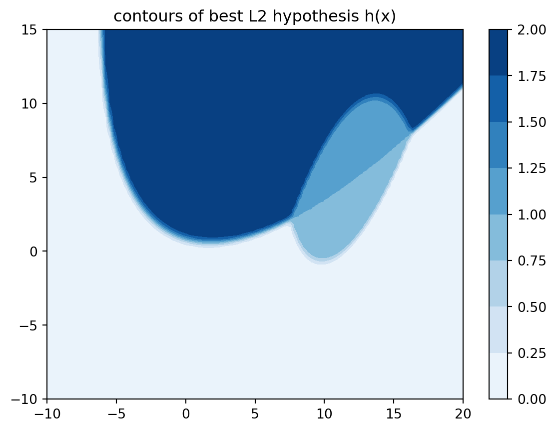
4.5 Bayes hypothesis for the \(L^2\) loss
By Theorem 3.3 from the lecture notes, a best hypothesis that minimizes the generalisation for the \(L^2\) loss is given by \[
h_\mathrm{best}(x) = \mathbb{E}[Y|X = x] \qquad (x \in \mathcal{X}).
\]
As \(Y\) is a discrete random variable, this reduces to a weighted sum \[
h_\mathrm{best}(x) = \sum_{i=0}^2 i\cdot \mathbb{P}(Y=i | X=x) = \frac{\sum_{i=0}^2 i \cdot \pi_i(x)/3}{\sum_{i=0}^2 \pi_i(x)/3}.
\]
The code below implements the Bayes hypothesis h_best_L2 and produces a contour plot. Note h_best_L2 does not necessarily attain integer values in \(\{0,1,2\}\). This might not be popular with the marketing department. Can you come up with a best possible hypothesis \(h\) that takes only values in \(\{0,1,2\}\)? Compute its generalisation error.
def h_best_L2(x): n, d =0, 0for i inrange(len(c_)): gd = gauss_density(x, c_[i], Sigma_[i]) n += i * gd d += gdreturn n/dx0 = np.linspace(-10, 20, 100)x1 = np.linspace(-10, 15, 100)X0, X1 = np.meshgrid(x0, x1)Z = np.zeros(X0.shape)for i inrange(X0.shape[0]):for j inrange(X0.shape[1]): x = np.array([X0[i, j], X1[i, j]]) Z[i, j] = h_best_L2(x)plt.contourf(X0, X1, Z, cmap=plt.cm.Blues);plt.title('contours of best L2 hypothesis h(x)');plt.colorbar();
We can also compute the generalisation error for h_best_L2 as shown below. (Note that we have replaced the infinite region in dblquad by a finite rectangle. The Gaussian densities decay fast enough for such a truncation to be valid.) As expected, it is smaller than what we got in Example 4.3 with the coordinate-split hypothesis. In fact, this is the Bayes error and no classifier can yield an \(L^2\) generalisation error that is below that.
Rh =0for i inrange(len(c_)): fun =lambda x1, x0: gauss_density(np.array([x0,x1]), c_[i], Sigma_[i]) * loss_L2(i, h_best_L2(np.array([x0,x1]))) # note x1, x0 order required by dblquad Rh += dblquad(fun, -10, 20, -10, 15)[0]/len(c_)print('generalisation error of best L2 hypothesis:', Rh)
generalisation error of best L2 hypothesis: 0.0018823084096411217
4.6 One-hot encoding
An attractive property of the squared \(L^2\) loss function is that there is a formula for an optimal hypothesis that minimizes the generalisation error. Unfortunately, encoding more than two classes using integer labels like we did above (recall, \(\mathcal{Y}=\{ 0,1,2\}\)) has a serious drawback: if, for example, a data point \((x,y)\) with label \(y=0\) is misclassified as a 1, this results in a squared \(L^2\) loss of \(L(0,1) = (1-0)^2=1\), whereas a misclassification of 0 as a 2 incurs a loss of \(L(0,2)=(2-0)^2=4\), i.e., much higher than we may intend. If we use such a loss function to train a machine learning model, the resulting model may put ‘overproportional effort’ in being accurate on labels 0 and 2, whilst neglecting data points with label 1 (as these can only be misclassified by one unit).
To overcome this issue and give equal weight to every misclassification, one uses a one-hot encoded label space \(\mathcal{Y}\) as follows: \[
\mathcal{Y} = \left\{ \begin{bmatrix} 1\\0\\0 \end{bmatrix}, \begin{bmatrix} 0\\1\\0 \end{bmatrix} , \begin{bmatrix} 0\\0\\1 \end{bmatrix} \right\}.
\] The optimal \(L^2\) hypothesis is then \[
h_\mathrm{best}(x) = \mathbb{E}[Y|X = x] = \begin{bmatrix} \pi_0(x) \\ \pi_1(x) \\\pi_2(x) \end{bmatrix} {\Large /} \sum_{i=0}^2 \pi_i(x).
\] The three entries of \(h_\mathrm{best}(x)\) can also be interpreted as levels of confidence we have in the assignment of \(x\) into any of the three classes.
def h_best_one_hot(x): y = np.zeros(len(c_))for i inrange(len(c_)): y[i] = gauss_density(x, c_[i], Sigma_[i])return y/np.sum(y)Rh =0for i inrange(len(c_)): one_hot = np.zeros(len(c_)) one_hot[i] =1 fun =lambda x1, x0: gauss_density(np.array([x0,x1]), c_[i], Sigma_[i]) * loss_L2(one_hot, h_best_one_hot(np.array([x0,x1]))) Rh += dblquad(fun, -10, 20, -10, 15)[0]/len(c_)print('generalisation error of best L2 hypothesis (one-hot encoding):', Rh)
generalisation error of best L2 hypothesis (one-hot encoding): 0.0011907288593209465
4.7 Rademacher complexity
Let us recall the definition of the empirical Rademacher complexity\[
\widehat{\rm Rad}({\bf G}) := \mathbb{E}\left[\sup_{g \in {\bf G}} \frac{1}{N}\sum_{n=1}^N \sigma_n g(x_n,y_n)\right],
\] for a space of hypothesis losses\[
{\bf G} := \big \lbrace g: g(x,y) = L(y,h(x)) \ ((x,y)\in \mathcal{Z}), h \in {\bf H}\big\rbrace.
\] The expectation \(\mathbb{E}\) is with respect to the i.i.d. Rademacher distributed random variables \(\sigma_1, \ldots, \sigma_N \sim \mathrm{Unif}(\{-1,+1\})\).
What is the intuition behind \(\widehat{\rm Rad}({\bf G})\)? Let’s fix for the moment one realisation of the \(\sigma_n\)’s. This partitions the data into two parts, those data points \((x_n,y_n)\) where \(\sigma_n=1\), and those where \(\sigma_n=-1\). In order to make the term inside the supremum large, we need to find a hypothesis \(h\in\mathbf{H}\) so that the loss \(L(y_n,h(x_n))\) is large on the data points where \(\sigma_n=+1\), and \(L(y_n,h(x_n))\) small when \(\sigma_n=-1\). In other words, the hypothesis is relatively accurate (has small error) on one part of the samples, and relatively inaccurate on the rest. This means that there is a hypothesis that can be misleadingly accurate for a subset of the data (e.g., some randomly selected training data) but leads to large generalisation error on some other subset. Or, we could say that this hypothesis overfits one subset of the data. If this is the case for every possible combination of data subsets, then the hypothesis space is “rich” (high complexity) and \(\widehat{\rm Rad}({\bf G})\) will be large.
Alternatively, if \(\widehat{\rm Rad}({\bf G})\) is small, then having a hypothesis that is accurate on a randomly selected subset of the data implies that, on average, that hypothesis is also accurate on the rest. In such a situation, we might say that the hypothesis generalises well, i.e., we expect to have a small generalisation error.
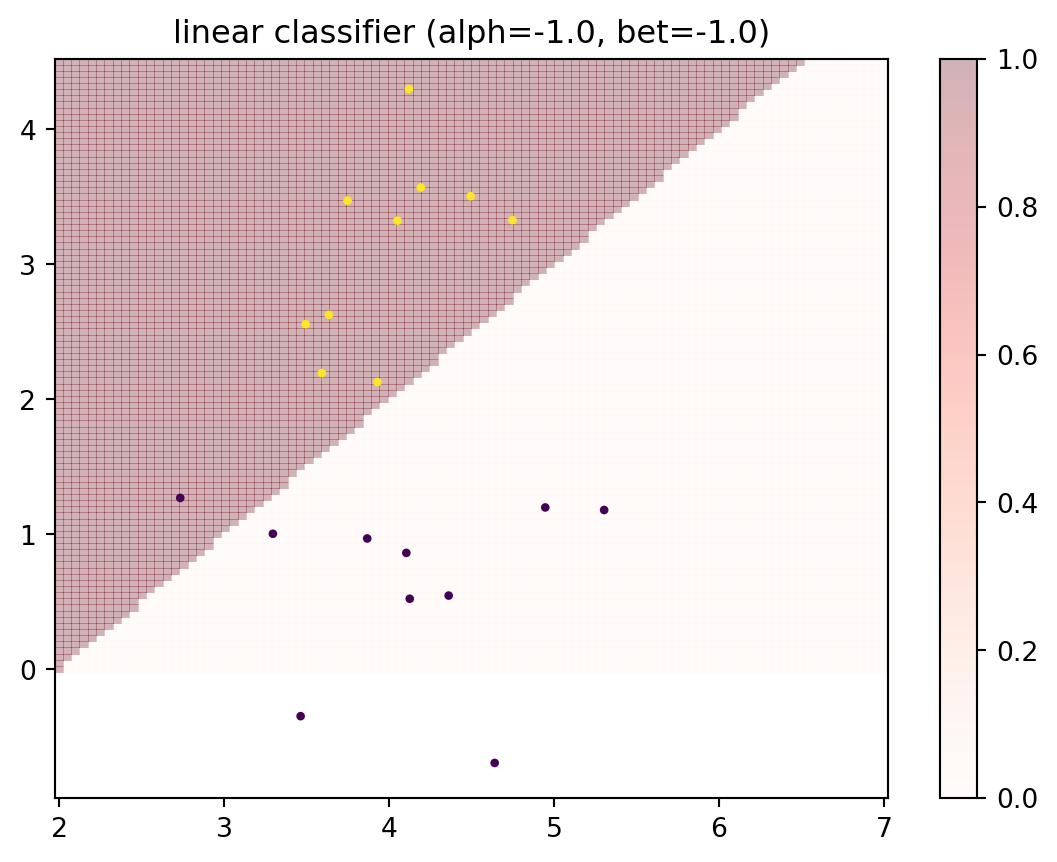
It is generally intractable to compute the empirical Rademacher complexity. Not least, because it would require averaging over all possible partitions of the data, of which there are \(2^N\), and then for each such partition, we would need to find the “most misleading” hypothesis. Nevertheless, for purpose of illustration, we can perform the following experiment. Consider a two-class classification problem with a small number of \(N=20\) data points. We will then consider two linear classifiers; one with a vertical decision boundary (i.e., just one parameter), and another with a fully linear decision boundary described by two parameters. Below is the setup for that.
def h_linear(x, alph, bet):""" linear classifier x0 + alph*x1 <= bet """ d = x[0,:] + alph*x[1,:] <= betreturn d.astype(int)# list of centers and covariance matrices for each classc_ = { 0: np.array([4, 1]), 1: np.array([4, 3])}Sigma_ = { 0: np.array([[1, 0.5], [0.5, 1]]), 1: np.array([[0.3, 0.2], [0.2, 0.8]]) }rng = default_rng(0)N =20X, y = multiple_classes(N, c_, Sigma_)# plot decision regions for these parametersalph =-1# -1...1bet =2# 2...7x0 = np.linspace(2, 7, 100)x1 = np.linspace(0, 4.5, 100)X0, X1 = np.meshgrid(x0, x1)Z = np.vstack((X0.flatten(),X1.flatten()))H = h_linear(Z,alph,bet).reshape(X0.shape)plt.pcolor(X0, X1, H, cmap=plt.cm.Reds, alpha=0.3);plt.title('linear classifier (alph={0:.1f}, bet={0:.1f})'.format(alph,bet));plt.colorbar();plt.scatter(X[0,:], X[1,:], s=5, c=y);# total loss of linear classifierhX = h_linear(X, alph, bet)print('total loss', np.sum(np.abs(hX - y)))
total loss 1.0
Given a realisation of the \(\sigma_n\), we will now maximise \(\sum_{n=1}^N \sigma_n g(x_n,y_n)\) over the parameters \((\alpha,\beta)\) that determine the decision boundary. In the first case, we will keep \(\alpha=0\) fixed and optimize for \(\beta\in[2,7]\), leading to a vertical decision boundary. In the second case we will optimize both \(\alpha\in [-1,1]\) and \(\beta\in[2,7]\). We will use a simple brute-force search to find the maximum of \(\frac{1}{N} \sum_{n=1}^N \sigma_n g(x_n,y_n)\), and display a table with the attained values.
Note
SciPy has a large collection of optimizers, including scipy.optimize.brute which implements brute-force search similar to what we’ve done below. As it’s so simple to do ourselves, we prefer our own implementation here.
print("sign pattern | one param | two params")loss =lambda alph, bet: np.abs(h_linear(X, alph, bet) - y)s0, s1 =0, 0for trial inrange(10):# realisation of Rademacher variables radem =2*rng.integers(2, size=N)-1# one parameter -> vertical decision boundary fun =lambda x: (1/N)*np.dot(radem, loss(0, x))# brute-force search for optimal paramater that maximises fun p0 = np.linspace(2, 7, 20) maxval0 =-np.inffor i inrange(len(p0)): maxval0 = np.max([fun(p0[i]),maxval0]) s0 += maxval0# two parameters -> linear decision boundary fun =lambda x: (1/N)*np.dot(radem, loss(x[0], x[1]))# brute-force search for optimal paramater that maximises fun p0 = np.linspace(-1, 1, 20) p1 = np.linspace(2, 7, 20) maxval1 =-np.inffor i inrange(len(p0)):for j inrange(len(p1)): maxval1 = np.max([fun([p0[i],p1[j]]),maxval1]) s1 += maxval1 sign =''.join([ ('+'if x >0else'-') for x in radem.tolist() ])print("{:20} | {:9.3f} | {:9.3f}".format(sign,maxval0,maxval1))print('='*(N+25))print("mean"+" "*(N-4) +" | {:9.3f} | {:9.3f}".format(s0/(trial+1),s1/(trial+1)))
We see that a larger value is achieved when we optimize over two parameters, instead of just one (not surprisingly). If we were to take the expectation of these values, as in the definition of the empirical Rademacher complexity, we’d obtain a larger expected value for the two-parameter case. This means that the two-parametric hypothesis space has a larger empirical Rademacher complexity than the one-parameter space.
4.7.1 Varying \(N\)
Recall from the lecture notes that there are probabilistic bounds on the Rademacher complexity \(R(h)\) using the empirical Rademacher complexity \(\tilde{R}(h)\); see, e.g., Corollary 3.16, which suggests \[
R(h) \leq \tilde{R}(h) + O\left(\sqrt{\frac{\log (N/d)}{N/d}} ; N \rightarrow \infty\right).
\] For such bounds to be meaningful, we demand that \(\tilde{R}(h)\) decreases as \(N\) increases. This is indeed the case as we verify by modifying the above code so that it prints out the averages for varying \(N\).
print(" N | one param | two params")rng = default_rng(0)for N in [20,50,100,200,1000,10000]: X, y = multiple_classes(N, c_, Sigma_) loss =lambda alph, bet: np.abs(h_linear(X, alph, bet) - y) s0, s1 =0, 0for trial inrange(100):# realisation of Rademacher variables radem =2*rng.integers(2, size=N)-1# one parameter -> vertical decision boundary fun =lambda x: (1/N)*np.dot(radem, loss(0, x))# brute-force search for optimal paramater that maximises fun p0 = np.linspace(2, 7, 20) maxval0 =-np.inffor i inrange(len(p0)): maxval0 = np.max([fun(p0[i]),maxval0]) s0 += maxval0# two parameters -> linear decision boundary fun =lambda x: (1/N)*np.dot(radem, loss(x[0], x[1]))# brute-force search for optimal paramater that maximises fun p0 = np.linspace(-1, 1, 20) p1 = np.linspace(2, 7, 20) maxval1 =-np.inffor i inrange(len(p0)):for j inrange(len(p1)): maxval1 = np.max([fun([p0[i],p1[j]]),maxval1]) s1 += maxval1print("{:9.0f} | {:9.3f} | {:9.3f}".format(N,s0/(trial+1),s1/(trial+1)))
We have learned that a larger hypothesis space \(\mathbf H\) will lead to a smaller approximation error defined as \[
\mathrm{approximation} := \inf_{h' \in \mathbf H} R(h') - R^{\mathrm Bayes}.
\] Recall that \(R^{\mathrm Bayes}\) is the irreducible error that a Bayes hypothesis would achieve. The approximation error describes how close the generalisation error of the best possible hypothesis in \(\mathbf H\) is relative to a Bayes hypothesis. Clearly, having a small approximation error is generally a good thing. In practice, we will try to identify a near-best hypothesis \(h \in \mathbf H\) by minimizing some empirical error on a finite dataset. Unfortunately, as the complexity of \(\mathbf H\) increases (the hypothesis space becomes more expressive), a hypothesis \(h\in\mathbf H\) can have increased tendency to fit too closely to the training data, and it may not generalise well to other data from the same distribution. As a consequence, it gets harder to identify (``estimate’’) a model \(h\) whose generalisation error \(R(h)\) is close to the best possible on the whole data. The difference between \(R(h)\) and the best possible is called the estimation error, \[
\mathrm{estimation} := R(h) - \inf_{h'\in \mathbf H} R(h').
\]
By the simple relation \[
R(h) = R^{\mathrm Bayes} + \mathrm{approximation} + \mathrm{estimation},
\] we can conclude the following: if enlarging the hypothesis space \(\mathbf H\) does not lead to a reduced generalisation error \(R(h)\), or even results in an increase of \(R(h)\), then necessarily the estimation error is no longer decreasing.
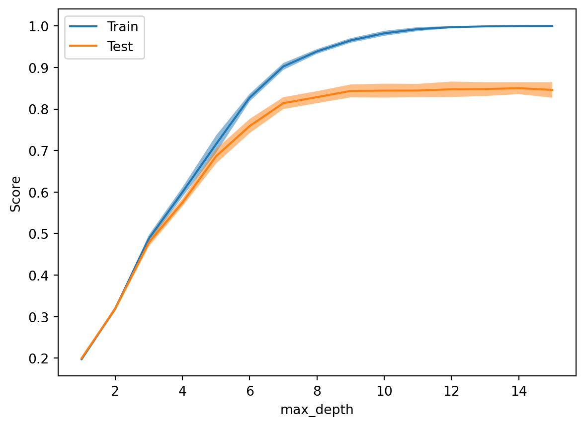
It is relatively difficult to construct a meaningful example to visualise the approximation-estimation trade-off. The below code uses a decision tree for classifying images of ten digits into classes \(\{0,1,\ldots,9\}\). The maximal tree depth is varied from 1 to 15. We observe that the error on the test set stagnates as the maximal tree depth exceeds about 7, while the approximation error on the train set continues decreasing. In that regime, we are overfitting the model to the training data and generalisation no longer improves. (If we randomly perturb some of the labels, we can even observe the test error to increase when the tree depth exceeds about 7.)
from sklearn import datasetsfrom sklearn.utils import shufflefrom sklearn.tree import DecisionTreeClassifierfrom sklearn.model_selection import train_test_splitimport numpy as npimport matplotlib.pyplot as pltds = datasets.load_digits()X, y = ds['data'], ds['target']X, y = shuffle(X, y, random_state=42)# try pollute ~10% of labels to test error increasing #y[0:180] = np.random.randint(0,10,180) X_train, X_test, y_train, y_test = train_test_split( X, y, test_size=0.3, random_state=42)loss_train = np.zeros(15)loss_test = np.zeros(15)depth = np.arange(1,16)for d in depth: tree = DecisionTreeClassifier(max_depth=d) tree.fit(X_train, y_train)# compute normalised train/test loss y_pred = tree.predict(X_train) loss_train[d-1] = np.sum(y_train!=y_pred)/y_train.shape[0] y_pred = tree.predict(X_test) loss_test[d-1] = np.sum(y_test!=y_pred)/y_test.shape[0]plt.plot(depth, loss_train, label='train loss')plt.plot(depth, loss_test, label='test loss')plt.xlabel('max tree depth'); plt.ylabel('normalised loss')plt.legend();
Note
Sklearn provides several functions to simplify studies like the above. See, for example, the following code:
from sklearn.model_selection import ValidationCurveDisplay, StratifiedShuffleSplitValidationCurveDisplay.from_estimator( DecisionTreeClassifier(), X, y, param_name="max_depth", param_range=range(1,16), cv=StratifiedShuffleSplit(n_splits=10, train_size=0.7, test_size=0.3, random_state=42));