Code
import numpy as np
from numpy.random import default_rng
import matplotlib.pyplot as plt
import numpy as np
import seaborn as sns
from time import time\[ \newcommand{\float}{\mathbb{F}} \newcommand{\real}{\mathbb{R}} \newcommand{\complex}{\mathbb{C}} \newcommand{\nat}{\mathbb{N}} \newcommand{\integer}{\mathbb{Z}} \newcommand{\bfa}{\mathbf{a}} \newcommand{\bfe}{\mathbf{e}} \newcommand{\bfh}{\mathbf{h}} \newcommand{\bfp}{\mathbf{p}} \newcommand{\bfq}{\mathbf{q}} \newcommand{\bfu}{\mathbf{u}} \newcommand{\bfv}{\mathbf{v}} \newcommand{\bfw}{\mathbf{w}} \newcommand{\bfx}{\mathbf{x}} \newcommand{\bfy}{\mathbf{y}} \newcommand{\bfz}{\mathbf{z}} \newcommand{\bfA}{\mathbf{A}} \newcommand{\bfW}{\mathbf{W}} \newcommand{\bfX}{\mathbf{X}} \newcommand{\bfzero}{\boldsymbol{0}} \newcommand{\bfmu}{\boldsymbol{\mu}} \newcommand{\TP}{\text{TP}} \newcommand{\TN}{\text{TN}} \newcommand{\FP}{\text{FP}} \newcommand{\FN}{\text{FN}} \newcommand{\rmn}[2]{\mathbb{R}^{#1 \times #2}} \newcommand{\dd}[2]{\frac{d #1}{d #2}} \newcommand{\pp}[2]{\frac{\partial #1}{\partial #2}} \newcommand{\norm}[1]{\left\lVert \mathstrut #1 \right\rVert} \newcommand{\abs}[1]{\left\lvert \mathstrut #1 \right\rvert} \newcommand{\twonorm}[1]{\norm{#1}_2} \newcommand{\onenorm}[1]{\norm{#1}_1} \newcommand{\infnorm}[1]{\norm{#1}_\infty} \newcommand{\innerprod}[2]{\langle #1,#2 \rangle} \newcommand{\pr}[1]{^{(#1)}} \newcommand{\diag}{\operatorname{diag}} \newcommand{\sign}{\operatorname{sign}} \newcommand{\dist}{\operatorname{dist}} \newcommand{\simil}{\operatorname{sim}} \newcommand{\ee}{\times 10^} \newcommand{\floor}[1]{\lfloor#1\rfloor} \newcommand{\argmin}{\operatorname{argmin}} \newcommand{\E}[1]{\operatorname{\mathbb{E}}\left[\mathstrut #1\right]} \newcommand{\Cov}{\operatorname{Cov}} \newcommand{\logit}{\operatorname{logit}} \]
import numpy as np
from numpy.random import default_rng
import matplotlib.pyplot as plt
import numpy as np
import seaborn as sns
from time import timeDeep learning refers to utilizing neural networks with multiple layers to perform tasks such as classification, regression, and representation learning. While scikit-learn provides some basic support for neural networks, it is not intended for large-scale computations. In particular, scikit-learn offers no support for graphical processing units (GPUs) or tensor processing units (TPUs), which are typically used to train deep neural networks.
In this chapter we will be using PyTorch, a popular machine learning library that supports computing with tensors (a fancy word for the multi-dimensional arrays available in NumPy) with GPU acceleration and an automatic differentiation system.
When training neural networks, the most frequently used algorithm is back propagation. In this algorithm, parameters (model weights) are adjusted according to the gradient of the loss function with respect to the given parameter.
To compute those gradients, PyTorch has a built-in differentiation engine called torch.autograd. It supports automatic computation of gradients for any computational graph.
Conceptually, autograd records all of the operations as the data passes through the neural network, giving a directed acyclic graph whose leaves are the input tensors and roots are the output tensors. By tracing this graph from roots to leaves, one can automatically compute the gradients using the chain rule.
Consider the simplest one-layer neural network \[ y = w^T x + b \] with input \(x\), parameters \(w\) and \(b\), and some loss function. This is indeed just a linear regressor. It can be defined in PyTorch in the following manner:
import torch
torch.manual_seed(seed=42)

x = torch.randn(5)  # input tensor
y = torch.randn(3)  # expected output
w = torch.randn(5, 3, requires_grad=True)
b = torch.randn(3, requires_grad=True)
z = torch.matmul(x, w) + b
L = torch.nn.functional.mse_loss(z, y) # loss
We can get the value of the loss function for the data that we have provided as a Python float:
L.item()2.430109977722168Displaying L reveals that this numerical value is stored as a tensor together with a function handle:
Ltensor(2.4301, grad_fn=<MseLossBackward0>)We can get the numerical values of all tensors as NumPy arrays and verify the loss manually:
z_np = np.matmul(x.numpy(), w.detach().numpy()) + b.detach().numpy()
L_np = np.mean((y.numpy() - z_np)**2)
L_np2.43011We need to call detach() on some of the tensors first to detach them from the computational graph before converting to NumPy (which does not track gradients).
The function handles grad_fn present in some tensors are used for the automatic computation of gradients in PyTorch. We normally do not need to access these functions ourselves. When PyTorch performs a forward calculation (as the evaluation of loss above), it forms a computational graph of the involved operations. Using the chain rule, this graph is used to compute gradients of L with respect to tensors that have been defined with the requires_grad=True property:
L.backward()
print("dL/db =", b.grad)
print("dL/dw ="); print(w.grad)
dL/db = tensor([-0.2143, -1.6107, 0.7745])
dL/dw =
tensor([[-0.0721, -0.5423, 0.2608],
[-0.0276, -0.2075, 0.0998],
[-0.0502, -0.3777, 0.1816],
[-0.0493, -0.3710, 0.1784],
[ 0.2406, 1.8086, -0.8696]])We can manually use these gradients to update the parameters using gradient descent:
lr = 0.5 # learning rate

for iter in range(5):

    # update weights b and w
    b.data = b.data - lr*b.grad
    w.data = w.data - lr*w.grad

    # reset gradient accumulators
    b.grad.zero_()
    w.grad.zero_()

    # forward feed
    z = torch.matmul(x, w) + b
    L = torch.nn.functional.mse_loss(z, y)
    print("iter =", iter, "   loss =", L.item())

    # backpropagate
    L.backward()
iter = 0 loss = 0.06783159077167511
iter = 1 loss = 0.0018933814717456698
iter = 2 loss = 5.284887447487563e-05
iter = 3 loss = 1.4753180721527315e-06
iter = 4 loss = 4.116877860838031e-08In that loop, we need to set the gradients with respect to \(b\) and \(w\) to zero after each iteration. Otherwise, PyTorch would accumulate all gradient contributions.
The power of PyTorch is that we can construct much more complicated models and loss functions, and use the same automatic differentiation framework to optimize parameters. Below we demonstrate the basic PyTorch workflow by building and training a neural network with multiple fully connected layers. The workflow includes loading and preparing the data, defining the neural network model, optimizing the model parameters, and making predictions.
PyTorch offers domain-specific libraries such as TorchText, TorchVision, and TorchAudio, all of which include datasets.
The torchvision.datasets module contains Dataset objects for many real-world vision data like CIFAR, COCO (full list here). Every TorchVision dataset includes two arguments: transform and target_transform to modify the samples and labels respectively. Here we use the FashionMNIST dataset.
import torch
from torch import nn
from torch.utils.data import DataLoader
from torchvision import datasets
from torchvision.transforms import ToTensor

# Download training data
training_data = datasets.FashionMNIST(root="deep_store", train=True,
                            download=True, transform=ToTensor())

# Download test data
test_data = datasets.FashionMNIST(root="deep_store", train=False,
                            download=True, transform=ToTensor())

classes = [ "T-shirt/top", "Trouser", "Pullover", "Dress", "Coat",
            "Sandal", "Shirt", "Sneaker", "Bag", "Ankle boot" ]
Here are the first 16 images in the training data and their respective labels.
fig, axes = plt.subplots(4,4)
fig.tight_layout()
for i in range(4):
    for j in range(4):
        k = j + 4*i
        x, y = training_data[k][0], training_data[k][1]
        img = x[0,:,:].data
        sns.heatmap(1-img,ax=axes[i,j],square=True,cmap="gray",cbar=False)
        axes[i,j].axis(False)
        axes[i,j].set_title(classes[y])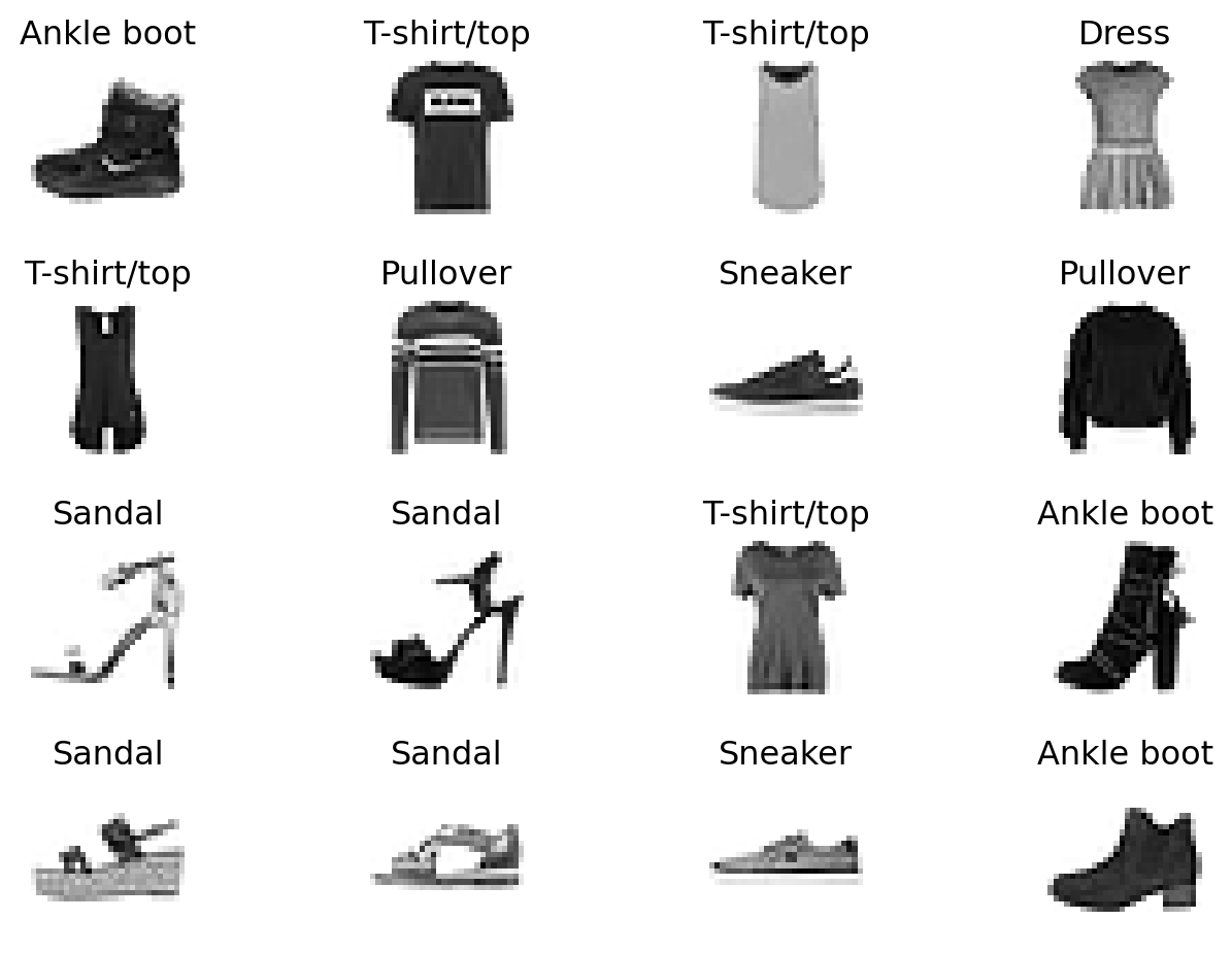
We pass the dataset as an argument to DataLoader. This wraps an iterable over our dataset, and supports automatic batching, sampling, shuffling, and multiprocess data loading. We define a batch size of 64, i.e., each element in the dataloader iterable will return a batch of 64 features and labels. The features of one batch are stored in a four-dimensional array of size batch size × number of input channels × image height × image width.
# Create data loaders
batch_size = 64
train_dataloader = DataLoader(training_data, batch_size=batch_size)
test_dataloader = DataLoader(test_data, batch_size=batch_size)

for X, y in test_dataloader:
    print(f"Shape of X [N, C, H, W]: {X.shape}")
    print(f"Shape of y: {y.shape} {y.dtype}")
    break
Shape of X [N, C, H, W]: torch.Size([64, 1, 28, 28])
Shape of y: torch.Size([64]) torch.int64To define a neural network in PyTorch, we create a class that inherits from nn.Module. We define the layers of the network in the __init__ function and specify how data will pass through the network in the forward function. To accelerate operations in the neural network, PyTorch can move it to an available GPU. Otherwise, it will use the CPU.
The network we define here is a multilayer perceptron with \(L=3\) layers, using the ReLu activation function on the first and second layers, each with 512 neurons. On the third layer we use the identity function \(\varphi(x)=x\), effectively implementing a linear mapping from an internal 512-dimensional space to the 10-dimensional label space (one-hot encoding of 10 labels).
# Get the best available device
if torch.cuda.is_available():
    device = torch.device("cuda")
    device_name = torch.cuda.get_device_name(0)
elif torch.backends.mps.is_available():
    device = torch.device("mps")
else:
    device = torch.device("cpu")

print(f"Using {device} device")

# Define the model
class NeuralNetwork(nn.Module):
    def __init__(self):
        super().__init__()
        self.flatten = nn.Flatten()
        self.linear_relu_stack = nn.Sequential(
            nn.Linear(28*28, 512),
            nn.ReLU(),
            nn.Linear(512, 512),
            nn.ReLU(),
            nn.Linear(512, 10)
        )

    def forward(self, x):
        x = self.flatten(x)
        logits = self.linear_relu_stack(x)
        return logits

# Instantiate and move the model to the device
torch.manual_seed(seed=42)
model = NeuralNetwork().to(device)
print(model)
Using cpu device
NeuralNetwork(
(flatten): Flatten(start_dim=1, end_dim=-1)
(linear_relu_stack): Sequential(
(0): Linear(in_features=784, out_features=512, bias=True)
(1): ReLU()
(2): Linear(in_features=512, out_features=512, bias=True)
(3): ReLU()
(4): Linear(in_features=512, out_features=10, bias=True)
)
)The parameters of the model are accessible via the parameters() method, and we can calculate the total number of trainable parameters as follows:
total_params = sum(p.numel() for p in model.parameters() if p.requires_grad)
print(f'Total number of parameters: {total_params}')
Total number of parameters: 669706That number corresponds to \((784+1)\times 512 + (512+1)\times 512 + (512+1)\times 10\), the total number of elements in the three weight matrices plus the entries of the bias vectors on each layer.
To train a model, we need a loss function and an optimizer.
loss_fn = nn.CrossEntropyLoss()
optimizer = torch.optim.SGD(model.parameters(), lr=1e-2)
In a single training loop, the model makes predictions on the training dataset (fed to it in batches), and backpropagates the prediction error to adjust the model’s parameters. The name SGD of the optimizer stands for stochastic gradient descent. This is a somewhat confusing name for the only randomness in that method comes from the fact that the training is performed on batches (in our case, batches of 64 feature-label pairs), compiled from the overall data by the DataLoader.
At each training step, the optimizer performs a deterministic gradient descent step to update all the weights, hopefully improving the loss function involving 64 additive terms for the data points in the batch. After cycling through the whole train set in batches, an epoch is completed and the optimizer got to “see” all the training data. (There is an optional shuffle=True argument that can be provided to the DataLoader. In that case, the batches vary from epoch to epoch.)
def train(dataloader, model, loss_fn, optimizer):
    size = len(dataloader.dataset)
    model.train() # switch to train mode
    for batch, (X, y) in enumerate(dataloader):
        X, y = X.to(device), y.to(device)

        # Compute prediction error
        pred = model(X)
        loss = loss_fn(pred, y)

        # Backpropagation
        loss.backward()
        optimizer.step()
        optimizer.zero_grad()

        if batch % 250 == 0:
            loss, current = loss.item(), (batch + 1) * len(X)
            print(f"loss: {loss:>7f}  [{current:>5d}/{size:>5d}]")
We also check the model’s performance against the test dataset to ensure it is learning.
def test(dataloader, model, loss_fn):
    size = len(dataloader.dataset)
    num_batches = len(dataloader)
    model.eval() # switch to evaluation mode
    test_loss, correct = 0, 0
    with torch.no_grad():
        for X, y in dataloader:
            X, y = X.to(device), y.to(device)
            pred = model(X)
            test_loss += loss_fn(pred, y).item()
            correct += (pred.argmax(1) == y).type(torch.float).sum().item()
    test_loss /= num_batches
    correct /= size
    print(f"Accuracy on test set: {(100*correct):>0.1f}%, Avg loss: {test_loss:>8f} \n")
The training process is conducted over several iterations (epochs). During each epoch, the model learns parameters to make better predictions. We print the model’s accuracy and loss at each epoch; we’d like to see the accuracy increase and the loss decrease with every epoch.
epochs = 3
st = time()
for t in range(epochs):
    print(f"Epoch {t+1}\n-------------------------------")
    train(train_dataloader, model, loss_fn, optimizer)
    test(test_dataloader, model, loss_fn)
print("Epochs completed in", time()-st, "seconds.")
Epoch 1
-------------------------------
loss: 2.298730 [ 64/60000]
loss: 1.726617 [16064/60000]
loss: 1.045534 [32064/60000]
loss: 0.713352 [48064/60000]
Accuracy on test set: 71.4%, Avg loss: 0.793634
Epoch 2
-------------------------------
loss: 0.801753 [ 64/60000]
loss: 0.794043 [16064/60000]
loss: 0.635068 [32064/60000]
loss: 0.518066 [48064/60000]
Accuracy on test set: 78.0%, Avg loss: 0.635894
Epoch 3
-------------------------------
loss: 0.573711 [ 64/60000]
loss: 0.699730 [16064/60000]
loss: 0.558132 [32064/60000]
loss: 0.470907 [48064/60000]
Accuracy on test set: 79.8%, Avg loss: 0.572663
Epochs completed in 15.694223880767822 seconds.The trained model can be used to make predictions. Here are the predictions on the first 16 images from the test set, with the correct predictions highlighted with an asterisk (*).
model.eval()

fig, axes = plt.subplots(4,4)
fig.tight_layout()
for i in range(4):
    for j in range(4):
        k = j + 4*i
        x, y = test_data[k][0], test_data[k][1]

        img = x[0,:,:].data
        sns.heatmap(1-img,ax=axes[i,j],square=True,cmap="gray",cbar=False)
        axes[i,j].axis(False)

        with torch.no_grad():
            # x is 1x32x32 but model normally expects a batch 1x1x32x32
            x = x.unsqueeze(0)
            x = x.to(device)
            pred = model(x)

        predicted, actual = classes[pred[0].argmax(0)], classes[y]
        if predicted == actual:
            predicted += '*'
        axes[i,j].set_title(predicted)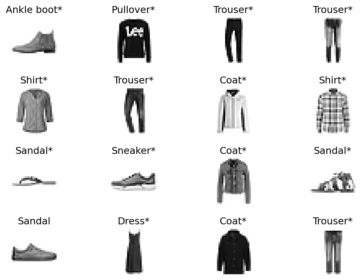
As training a neural network models can take quite a bit of time, it’s often useful to be able to save and load trained models. A common way to save a model is to serialize the internal state dictionary (containing the model parameters). The process for loading a model includes recreating the model structure and loading the state dictionary into it.
# saving to file model.pth
torch.save(model.state_dict(), "model.pth")

# loading
model = NeuralNetwork().to(device) # must be available
model.load_state_dict(torch.load("model.pth", weights_only=True))
<All keys matched successfully>Training and making predictions with large neural networks and datasets can be computationally intensive. Usually, these computations are not performed on CPUs (central processing units) as are available on your computer but on GPUs (graphical processing units) or TPUs (tensor processing units).
If you do not have GPU/TPU hardware for training your models, you can rent them from a cloud computing provider. Some popular providers include:
Amazon Web Services (AWS): AWS offers GPU instances through its EC2 (Elastic Cloud) service. The p3 and g4 instance types are commonly used for machine learning tasks.
Google Cloud Platform (GCP): GCP provides GPUs and TPUs for machine learning workloads. The AI Platform and Vertex AI are tailored for ML tasks.
Microsoft Azure: Azure offers GPU-enabled virtual machines, such as the NC and ND series, for deep learning and other compute-intensive tasks.
NVIDIA GPU Cloud (NGC): NVIDIA provides pre-configured GPU instances optimized for deep learning workloads.
Paperspace: Paperspace offers GPU instances and a platform called Gradient for running Jupyter notebooks and training models.
Google Colab: A free option for smaller projects, Google Colab provides access to GPUs and TPUs for training models in Jupyter notebooks.
When using cloud computing, you typically upload your data and code to the cloud, configure the hardware resources, and then run your training jobs. After training, you can download the trained model or deploy it directly from the cloud. Most cloud providers make VS Code extensions available to manage your code and data on the cloud infrastructure, but it is also possible to access these services from a browser.
If you just ant to try out some basic GPU training on a medium-sezed dataset for free, Google Colab is a good choice.
The PyTorch framework is very general: as long as we can define a neural network model that maps (batches of) data to a scalar loss function, PyTorch will take care of computing gradients with respect to the model’s parameters and provide powerful optimizers to reduce the empirical loss. Below we discuss some specialised neural network architectures that are commonly used.
A particularly useful and widespread architecture for image data is the class of convolutional neural networks, or CNN. In these, many of the linear maps in each layer correspond to the mathematical operation of convolution. These are then usually combined with activation functions, pooling layers, and fully connected layers.
In the context of functions, the convolution of two real-valued functions \(f\) and \(g\) is defined as the function \[ f * g(y) = \int_{-\infty}^\infty f(x) \cdot g(y-x) \mathrm{d}x. \] In a discrete setting, given a vector \(x\in\mathbb{R}^d\) and a sequence \(g = [ g_{-d+1},\ldots, g_{d-1}]^T\), the convolution is defined as the vector \(y = [y_1,\ldots, y_d]^T\) with \[ y_k = \sum_{i=1}^d x_i g_{k-i}, \quad k = 1,\ldots, d. \]
In matrix form: \[ \begin{pmatrix} y_1 \\ y_2 \\ \vdots \\ y_d \end{pmatrix} = \begin{pmatrix} g_0 & g_{-1} & \cdots & g_{-d+1} \\ g_1 & g_0 & \cdots & g_{-d+2} \\ \vdots & \vdots & \ddots & \vdots \\ g_{d-1} & g_{d-2} & \cdots & g_0 \end{pmatrix} \begin{pmatrix} x_1 \\ x_2 \\ \vdots \\ x_d \end{pmatrix}. \] The sequence \(g\) is called a filter in signal processing. Typically, multiplying a \(d \times d\) matrix with a \(d\)-dimensional vector requires \(d^2\) multiplications. If, however, the matrix has a special structure, then it is possible to perform this multiplication much faster, without having to explicitly represent the matrix as two-dimensional array in memory.
Example: The cyclic convolution corresponds to multiplication with a circulant matrix: \[ C = \begin{pmatrix} c_0 & c_1 & \cdots & c_{d-1} \\ c_{d-1} & c_0 & \cdots & c_{d-2} \\ \vdots & \vdots & \ddots & \vdots \\ c_1 & c_2 & \cdots & c_0 \end{pmatrix}. \] This is the same as the convolution with a sequence \(g\) as above, with \(c_i = g_{−i}\) and \(g_i = g_{d−1}\) for \(i = 1,\ldots,d-1\). A special case of a circulant matrix is the Discrete Fourier Transform (DFT), in which \(c_{jk} = \exp(2\pi i \cdot jk / n)\).
The DFT plays an important role in signal and image processing, and versions of it, such as the two-dimensional discrete cosine transform (DCT-2D), are the basis of the image compression standard JPEG. One of the most influential and widely used algorithms, the fast fourier transform (FFT), computes a DFT with \(O(d \log(d))\) operations, and this is essentially optimal. FFT-based algorithms can also be applied to carry out cyclic convolutions, since circulants are diagonalized by DFT matrices.
Example: In many applications, only a few of the entries of \(g\) will be non-zero. Perhaps the easiest and most illustrative example is the difference matrix \[ D = \begin{pmatrix} -1 & 1 & 0 & \cdots & 0 \\ 0 & -1 & 1 & \cdots & 0 \\ \vdots & \vdots & \ddots & \ddots & \vdots \\ 0 & 0 & \cdots & -1 & 1 \\ 0 & 0 & \cdots & 0 & -1 \end{pmatrix}. \]
This matrix maps a vector \(x\) to the vector of differences \(x_{i+1} − x_i\). This transformation detects changes in the vector, and a vector that is constant over a large range of coordinates is mapped to a sparse vector. Again, computing \(y = Dx\) requires just \(d − 1\) subtractions and no multiplications, and it is not necessary to store \(D\) as matrix in memory.
Given a convolution \(G\), one often only considers a subset of the rows, such as every second or every third row. If only every \(k\)-th row is considered, then we say that the filter has stride length \(k\). If the support (the number of non-zero entries) of \(g\) is small, then one can interpret the convolution operation as taking the inner product of \(g\) with a particular section of \(x\), and then moving this section, or “window”, by \(k\) entries if the stride length is \(k\). Each such operation can be seen as extracting certain information from a part of \(x\).
In the context of colour image data, the vector \(x\) will not be seen as a single vector in some \(\mathbb{R}^d\), but as a tensor with format \(3\times N \times M\). Here, the image is considered to be a \(N \times M\) matrix, with each entry corresponding to a pixel, and each pixel is represented by a 3-tuple consisting of the red, blue, and green components. A convolution filter will therefore operate on a subset of this tensor, typically a \(3 \times n \times m\) window. Typical parameters are \(N = M = 28\) and \(n = m = 5\). Each \(3 \times 5 \times 5\) block is mapped linearly to an entry of a \(24\times 24\) matrix in the same way (that is, applying the same filter).
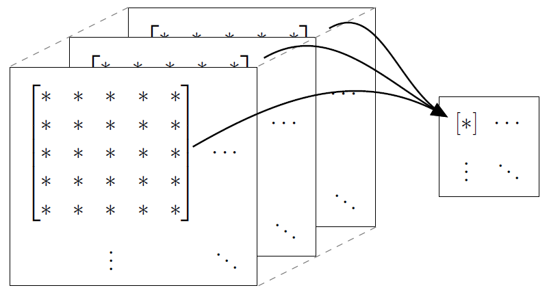
The filter applied is called a kernel and the resulting map is interpreted as representing a feature. Specifically, instead of writing it as a vector \(g\), we can write it as a matrix \(K\), and then have, if we denote the input image by \(X\), \[ Y = X * K, \quad Y_{ij} = \sum_{k,\ell} X_{k\ell} \cdot K_{i-k,j-\ell}. \] The reason for the reduction from image size \(28\times 28\) to \(24\times 24\) in the above example is that we can’t center the convolution at the boundary of the image. In order to avoid this, it is common to apply some padding to the image by artificially enlarging it (e.g., with zero pixel values).
In a convolutional layer, various different kernels or convolutions are applied to the image. This can be seen as extracting several features from an image. Convolutional layers are often combined with pooling layers. In a pooling layer, a few entries (e.g., a \(4 \times 4\) submatrix) are combined into one entry, either by taking the maximum (max pooling) or by averaging. This operation reduces the size of the data. In addition, towards the end one often adds one or multiple fully connected layers.
One of the earliest demonstration of the effectiveness of convolutional layers in neural networks is the LeNet model. This model was developed to solve the MNIST classification problem. The model below has two convolutional layers and three fully connected layers to make up five trainable layers in total. It is well-known under the name LeNet-5.
class LeNet5(nn.Module):
    def __init__(self):
        super().__init__()
        self.conv1 = nn.Conv2d(1, 6, kernel_size=5, stride=1, padding=2)
        self.act = nn.Tanh()
        self.pool = nn.AvgPool2d(kernel_size=2, stride=2)
        self.conv2 = nn.Conv2d(6, 16, kernel_size=5, stride=1, padding=0)
        self.flat = nn.Flatten()
        self.fc1 = nn.Linear(400, 120)
        self.fc2 = nn.Linear(120, 84)
        self.fc3 = nn.Linear(84, 10)

    def forward(self, x):
        # input 1x28x28, output 6x28x28
        x = self.act(self.conv1(x))
        # input 6x28x28, output 6x14x14
        x = self.pool(x)
        # input 6x14x14, output 16x10x10
        x = self.act(self.conv2(x))
        # input 16x10x10, output 16x5x5
        x = self.pool(x)
        # input 16x5x5, output 400
        x = self.flat(x)
        # input 400, output 120
        x = self.act(self.fc1(x))
        # input 120, output 84
        x = self.act(self.fc2(x))
        # input 84, output 10
        x = self.fc3(x)
        return x

torch.manual_seed(seed=42)
model = LeNet5().to(device)
print(model, "\n")

total_params = sum(p.numel() for p in model.parameters() if p.requires_grad)
print(f'Total number of parameters: {total_params}')
LeNet5(
(conv1): Conv2d(1, 6, kernel_size=(5, 5), stride=(1, 1), padding=(2, 2))
(act): Tanh()
(pool): AvgPool2d(kernel_size=2, stride=2, padding=0)
(conv2): Conv2d(6, 16, kernel_size=(5, 5), stride=(1, 1))
(flat): Flatten(start_dim=1, end_dim=-1)
(fc1): Linear(in_features=400, out_features=120, bias=True)
(fc2): Linear(in_features=120, out_features=84, bias=True)
(fc3): Linear(in_features=84, out_features=10, bias=True)
)
Total number of parameters: 61706We can reuse the above defined functions train() and test() on this modified network architecture. Instead of SGD, we try another popular optimizer called Adam.
loss_fn = nn.CrossEntropyLoss() # as before
optimizer = torch.optim.Adam(model.parameters()) # Adam optimizer

epochs = 3
st = time()
for t in range(epochs):
    print(f"Epoch {t+1}\n-------------------------------")
    train(train_dataloader, model, loss_fn, optimizer)
    test(test_dataloader, model, loss_fn)
print("Epochs completed in", time()-st, "seconds.")
Epoch 1
-------------------------------
loss: 2.292280 [ 64/60000]
loss: 0.762693 [16064/60000]
loss: 0.492685 [32064/60000]
loss: 0.422695 [48064/60000]
Accuracy on test set: 82.5%, Avg loss: 0.471835
Epoch 2
-------------------------------
loss: 0.373341 [ 64/60000]
loss: 0.592566 [16064/60000]
loss: 0.375745 [32064/60000]
loss: 0.405109 [48064/60000]
Accuracy on test set: 84.9%, Avg loss: 0.403741
Epoch 3
-------------------------------
loss: 0.291001 [ 64/60000]
loss: 0.544265 [16064/60000]
loss: 0.338981 [32064/60000]
loss: 0.389095 [48064/60000]
Accuracy on test set: 85.9%, Avg loss: 0.372932
Epochs completed in 31.664655685424805 seconds.Just as convolutional neural networks are designed for image classification tasks, recurrent neural networks (RNNs) are a class of neural networks designed to operate on sequences. The defining feature of a RNN is memory: when processing an element from a sequence, the network takes into account conclusions drawn from previous elements in the same sequence. Applications of recurrent neural networks include speech recognition, handwriting recognition, text-to-speech synthesis, machine translation, sentiment analysis, and generating literature or music.
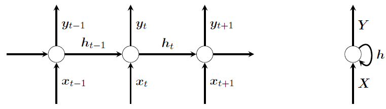
Recurrent neural networks operate on sequences \[ X = \{x_t \}_{t\geq 1}, \] where \(x_t \in \mathbb{R}^m\) for \(t \geq 1\). It is important to keep in mind that every sequence \(X\) is a data point in its own right, and not a collection of data points. Training data thus consists of a collection of sequences \(\{X_i\}_{i=1}^n\), and the network treats each such sequence as an individual input. In practice, such a sequence has finite length, but we do not need to bound the length explicitly here. The index \(t\) is suggestive of time, and will usually be referred to as such, but the data need not be a time series.
A general RNN can be described as \[ \begin{align} z_t &= W x_t + V h_{t-1} + b \\ y_t &= \rho(z_t) \\ h_t &= f(y_t, h_{t-1}), \end{align} \] where \(y_t\) are vectors forming the output sequence, \(h_t\) is referred to as the hidden state, and \(\rho, f\) are functions. Usually, the hidden state is initialized as \(h_0 = 0\). Of course, the output sequence of one RNN can be fed as an input in another, giving rise to multilayer RNNs.
There are several ways RNN architectures can be used, depending on the application. Here are a few examples.
Many-to-many: Feed in a sequence \(x_1,x_2,\ldots\) and use the whole output sequence \(y_1,y_2,\ldots\). This is can be applied, e.g., for machine translation or text generation.
Many-to-one: Feed in a sequence \(x_1,x_2,\ldots\) and use the final hidden state vector as a feature. This can be applied, e.g., for text classification and sentiment analysis.
One-to-many: Feed in single input \(x_1\) (e.g., repeatedly as \(x_1,x_1,\ldots\)) and use the whole output sequence \(y_1,y_2,\ldots\). This can be applied, e.g., for image annotation.
Below is PyTorch implementation of a simple character-level RNN trained on some of Shakespeare’s works. The input sequences \(X = \{ X_t\}\) consist of 100 hot-one encoded consecutive characters from the text, and the output sequences \(Y = \{ Y_t\}\) are one character advanced in the text. That is, the model learns to predict the next character in a sequence. The used RNN type is a three-layer long short-term memory (LSTM) architecture. After every epoch, the code produces 200 character predictions beginning with an arbitrarily chosen letter.
Note that, for performance reasons, the below cose only uses the first 50,000 characters from the text file _datasets/shakespeare.txt, and it starts with a pretrained model.
import torch
import torch.nn as nn
import torch.nn.functional as F
from torch.distributions import Categorical
import numpy as np
from tqdm import tqdm

# Get the best available device
if torch.cuda.is_available():
    device = torch.device("cuda")
    device_name = torch.cuda.get_device_name(0)
elif torch.backends.mps.is_available():
    device = torch.device("mps")
else:
    device = torch.device("cpu")
print(f"Using {device} device")

class RNN(nn.Module):
    def __init__(self, input_size, output_size, hidden_size, num_layers):
        super(RNN, self).__init__()
        self.embedding = nn.Embedding(input_size, input_size)
        self.rnn = nn.LSTM(input_size=input_size, hidden_size=hidden_size, num_layers=num_layers)
        self.decoder = nn.Linear(hidden_size, output_size)

    def forward(self, input_seq, hidden_state):
        embedding = self.embedding(input_seq)
        output, hidden_state = self.rnn(embedding, hidden_state)
        output = self.decoder(output)
        return output, (hidden_state[0].detach(), hidden_state[1].detach())

########### Hyperparameters ###########
hidden_size = 512   # size of hidden state
seq_len = 100       # length of input training sequence
num_layers = 3      # num of layers in LSTM layer stack
lr = 0.002          # learning rate
epochs = 2          # max number of epochs
op_seq_len = 200    # total num of characters in output test sequence
load_chk = True     # load weights from save_path directory to continue training
save_path = "./deep_store/CharRNN_shakespeare_50000.pth"
data_path = "./_datasets/shakespeare.txt"
#######################################

# load the text file
data = open(data_path, 'r').read()
data = data[:50000]   # truncate for speed
chars = sorted(list(set(data)))
data_size, vocab_size = len(data), len(chars)
print("----------------------------------------")
print("Data has {} characters, {} unique".format(data_size, vocab_size))
print("----------------------------------------")

# char to index and index to char maps
char_to_ix = { ch:i for i,ch in enumerate(chars) }
ix_to_char = { i:ch for i,ch in enumerate(chars) }

# convert data from chars to indices
data = list(data)
for i, ch in enumerate(data):
    data[i] = char_to_ix[ch]

# data tensor on device
data = torch.tensor(data).to(device)
data = torch.unsqueeze(data, dim=1)

# model instance
rnn = RNN(vocab_size, vocab_size, hidden_size, num_layers).to(device)

# load checkpoint if True
if load_chk:
    rnn.load_state_dict(torch.load(save_path))
    print("Pretrained model loaded successfully")
    print("----------------------------------------")

# loss function and optimizer
loss_fn = nn.CrossEntropyLoss()
optimizer = torch.optim.Adam(rnn.parameters(), lr=lr)

# training loop
print("Training")
for i_epoch in range(1, epochs+1):

    # random starting point (1st 100 chars) from data to begin
    data_ptr = np.random.randint(100)
    n = 0
    running_loss = 0
    hidden_state = None

    pbar = tqdm(total=data_size, position=0, leave=True);
    while True:

        pbar.update(seq_len)

        input_seq = data[data_ptr : data_ptr+seq_len]
        target_seq = data[data_ptr+1 : data_ptr+seq_len+1]

        # forward pass
        output, hidden_state = rnn(input_seq, hidden_state)

        # compute loss
        loss = loss_fn(torch.squeeze(output), torch.squeeze(target_seq))
        running_loss += loss.item()

        # compute gradients and take optimizer step
        optimizer.zero_grad()
        loss.backward()
        optimizer.step()

        # update the data pointer
        data_ptr += seq_len
        n +=1

        # if at end of data : break
        if data_ptr + seq_len + 1 > data_size:
            break

    pbar.close()

    # print loss and save weights after every epoch
    print("Epoch: {0} \t Loss: {1:.8f}".format(i_epoch, running_loss/n))
    torch.save(rnn.state_dict(), save_path)

    # sample / generate a text sequence after every epoch
    data_ptr = 0
    hidden_state = None

    # random character from data to begin
    rand_index = np.random.randint(data_size-1)
    input_seq = data[rand_index : rand_index+1]

    print("----------------------------------------")
    while True:
        # forward pass
        output, hidden_state = rnn(input_seq, hidden_state)

        # construct categorical distribution and sample a character
        output = F.softmax(torch.squeeze(output), dim=0)
        dist = Categorical(output)
        index = dist.sample()

        # print the sampled character
        print(ix_to_char[index.item()], end='')

        # next input is current output
        input_seq[0][0] = index.item()
        data_ptr += 1

        if data_ptr > op_seq_len:
            break

    print("\n----------------------------------------")
Using cpu device
----------------------------------------
Data has 50000 characters, 59 unique
----------------------------------------
Pretrained model loaded successfully
----------------------------------------
TrainingEpoch: 1 Loss: 0.78978641
----------------------------------------
e,
If are of thing way, to repett to doescefity,
For him ouf will do thring to die thought.
First Citizen:
Having not be daius, ang men hate me.
First Citizen:
No most fight.
BRUTUS:
Marcius, if thi
----------------------------------------Epoch: 2 Loss: 0.70239985
----------------------------------------
eed; to remember
vive it been consul, and leaves for
a peary at.
CORIOLUNUS:
Come,
Shall tood reports,
Afe his not country: look not many deee this mistoing
Of the matter?
First Citizen:
Fame not cou
----------------------------------------Transformers are a type of neural network architecture introduced in the paper “Attention is All You Need” by Vaswani et al. in 2017. They are designed to handle sequential data, such as text, and have become the foundation for many state-of-the-art models in natural language processing (NLP), including BERT, GPT, and T5.
The key innovation of transformers is the self-attention mechanism, which allows the model to weigh the importance of different words in a sequence relative to each other. This enables transformers to capture long-range dependencies in data more effectively than traditional recurrent neural networks (RNNs) or convolutional neural networks (CNNs).
Transformers consist of an encoder-decoder structure: - The encoder processes the input sequence and generates a set of representations. - The decoder uses these representations to generate the output sequence.
Transformers are highly parallelizable and efficient, making them suitable for large-scale training on modern hardware. They have revolutionized NLP and are also being applied to other domains like computer vision and reinforcement learning.
While we do not discuss transformers any further, we refer to its PyTorch implementation and an excellent video introduction.
There are various excellent sources and tutorials on deep learning available online.
Ian Goodfellow, Yoshua Bengio, and Aaron Courville. Deep Learning. MIT Press, 2016. http://www.deeplearningbook.org. [See in particular Chapter 9 on CNNs].
Catherine F. Higham and Desmond J. Higham. Deep learning: An introduction for applied mathematicians. SIAM Review, 61(4):860–891, 2019. [See in particular Chapter 7 which also contains a worked through CNN example in MATLAB.]
Martin Lotz. Mathematics of Machine Learning. University of Warwick lecture notes. [Great resource that has been followed for the sections on CNNs and RNNs.]
Aston Zhang, Zack C. Lipton, Mu Li, and Alex J. Smola. Dive into Deep Learning. Cambridge University Press, 2023.
PyTorch tutorials such as Classification of CIFAR10 images