This worksheet is based on the seventh lecture of the Statistical Modelling in Stata course, created by Dr Mark Lunt and offered by the Centre for Epidemiology Versus Arthritis at the University of Manchester. The original Stata exercises and solutions are here translated into their R equivalents.
Refer to the original slides and Stata worksheets here.
Cross-tabulation and logistic regression
Use the dataset epicourse.csv.
epicourse <- read.csv('epicourse.csv')
Produce a table of hip pain by gender using the table() function. What is the prevalance of hip pain in men and in women?
Generate a table of counts using
And you can convert this into a table of proportions within each sex (2nd margin) using:
prop.table(hip_tab, margin = 2)
     sex
hip_p          F          M
  no  0.84770485 0.90155678
  yes 0.15229515 0.09844322
In R 4.0.0, you can also use the new proportions() function.
proportions(hip_tab, margin = 2)
     sex
hip_p          F          M
  no  0.84770485 0.90155678
  yes 0.15229515 0.09844322
Perform a chi-squared test to test the hypothesis that there is a different prevalence of hip pain in men versus women.
chisq.test(hip_tab)
    Pearson's Chi-squared test with Yates' continuity correction

data:  hip_tab
X-squared = 29.158, df = 1, p-value = 6.672e-08
Obtain the odds ratio for being female compared to being male. What is the confidence interval for this odds ratio?
Recall the formula for an odds ratio is \[\text{OR} = \frac{D_E / H_E}{D_N / H_N},\] where \(D\) denotes ‘diseased’, \(H\) is ‘healthy’, \(E\) is ‘exposed’ (i.e. female) and \(N\) is ‘not exposed’ (i.e. male).
odds_ratio <- (hip_tab['yes', 'F'] / hip_tab['no', 'F']) /
  (hip_tab['yes', 'M'] / hip_tab['no', 'M'])
odds_ratio
[1] 1.645314And the Wald 95% confidence interval for the odds ratio given by \[\exp \left\{ \log \text{OR}~\pm~z_{\alpha/2} \times \sqrt{\tfrac1{D_E} + \tfrac1{D_N} +\tfrac1{H_E} + \tfrac1{H_N}} \right\},\] where \(z_{\alpha/2}\) is the critical value of the standard normal distribution at the \(\alpha\) significance level. In R, this interval can be computed as follows:
How does the odds ratio compare to the relative risk?
The relative risk is \[\text{RR} = \frac{D_E / N_E}{D_N / N_N},\] where \(N_E = D_E + H_E\) and \(N_N = D_N + H_N\) are the respective total number of exposed (female) and not-exposed (male) people in the sample. In R, it is
rel_risk <- hip_tab['yes', 'F'] / colSums(hip_tab)['F'] /
  (hip_tab['yes', 'M'] / colSums(hip_tab)['M'])
rel_risk
       F
1.547035
which is similar to the odds ratio.
Does the confidence interval for the odds ratio suggest that hip pain is more common in one of the sexes?
Yes, it suggests hip pain is more common in women, because the confidence interval does not contain 1.
I can’t see any point in computing a relative risk confidence interval here, even if the Stata command cs reports it.
Now fit a logistic regression model to calculate the odds ratio for being female, using the glm function. How does the result compare to that computed above?
Note. The glm function needs responses to be between 0 and 1, so it won’t work with a character vector of ‘yes’ and ‘no’. An easy solution is to replace hip_p with TRUE and FALSE (which in R is the same as 1 and 0). Either do this before fitting the model, or inline:
Call:
glm(formula = hip_p == "yes" ~ sex, family = binomial("logit"),
    data = epicourse)

Deviance Residuals:
    Min       1Q   Median       3Q      Max
-0.5748  -0.5748  -0.4553  -0.4553   2.1533

Coefficients:
            Estimate Std. Error z value Pr(>|z|)
(Intercept) -1.71671    0.05765 -29.781  < 2e-16 ***
sexM        -0.49793    0.09209  -5.407 6.41e-08 ***
---
Signif. codes:  0 '***' 0.001 '**' 0.01 '*' 0.05 '.' 0.1 ' ' 1

(Dispersion parameter for binomial family taken to be 1)

    Null deviance: 3424.1  on 4514  degrees of freedom
Residual deviance: 3394.1  on 4513  degrees of freedom
AIC: 3398.1

Number of Fisher Scoring iterations: 4
In this model, the intercept parameter estimate represents the log-odds of having hip pain, for women (taken to be the baseline). The sexM is the additive effect (to these log-odds) from being a man. Thus the odds ratio is simply the exponential of the negation of this second parameter:
and this is the same as the value calculated above.
How does the confidence interval compare to that calculated above?
Same as above (just reversed, because female is the baseline in the model).
Introducing continuous variables
Age may well affect the prevalence of hip pain, as well as gender. To test this, create an agegroup variable with the following code:
Tabulate hip pain against age group with the table() function. Is there evidence that the prevalence of hip pain increases with age?
     agegroup
hip_p (0,30] (30,40] (40,50] (50,60] (60,70] (70,80] (80,90]
  no     423     353     534     484     792     965     362
yes 10 13 55 86 158 176 63chisq.test(age_tab)
    Pearson's Chi-squared test

data:  age_tab
X-squared = 102.35, df = 6, p-value < 2.2e-16
There is evidence that the prevalence changes with age, however the test does not actually tell us the pattern or sign of the effect.
Add age to the logistic regression model for hip pain. Is age a significant predictor of hip pain?
You can rewrite the model from scratch with glm(), or use this convenient shorthand:
Call:
glm(formula = hip_p == "yes" ~ sex + age, family = binomial("logit"),
    data = epicourse)

Deviance Residuals:
    Min       1Q   Median       3Q      Max
-0.8441  -0.5684  -0.4801  -0.3639   2.6272

Coefficients:
             Estimate Std. Error z value Pr(>|z|)
(Intercept) -3.326800   0.192175 -17.311  < 2e-16 ***
sexM        -0.530815   0.093057  -5.704 1.17e-08 ***
age          0.025813   0.002808   9.193  < 2e-16 ***
---
Signif. codes:  0 '***' 0.001 '**' 0.01 '*' 0.05 '.' 0.1 ' ' 1

(Dispersion parameter for binomial family taken to be 1)

    Null deviance: 3424.1  on 4514  degrees of freedom
Residual deviance: 3298.9  on 4512  degrees of freedom
AIC: 3304.9

Number of Fisher Scoring iterations: 5
It looks like the age coefficient is statistically significant.
How do the odds of having hip pain change when age increases by one year?
It is a logistic model, so the parameter estimate represents the increase in log-odds for one year increase in age.
Thus odds of hip pain increase by 1.03 for each year increase in age.
Fit an appropriate model to test whether the effect of age differs between men and women.
Call:
glm(formula = hip_p == "yes" ~ age * sex, family = binomial,
    data = epicourse)

Deviance Residuals:
    Min       1Q   Median       3Q      Max
-0.8812  -0.5540  -0.4730  -0.3643   2.5245

Coefficients:
             Estimate Std. Error z value Pr(>|z|)
(Intercept) -3.548531   0.244116 -14.536  < 2e-16 ***
age          0.029195   0.003598   8.115 4.85e-16 ***
sexM         0.060534   0.387861   0.156    0.876
age:sexM    -0.008986   0.005742  -1.565    0.118
---
Signif. codes:  0 '***' 0.001 '**' 0.01 '*' 0.05 '.' 0.1 ' ' 1

(Dispersion parameter for binomial family taken to be 1)

    Null deviance: 3424.1  on 4514  degrees of freedom
Residual deviance: 3296.5  on 4511  degrees of freedom
AIC: 3304.5

Number of Fisher Scoring iterations: 5
The interaction term (age:sexM) is not significant, so men and women do not have different slopes in the model; the effect of advancing in age is not different between men and women.
Rather than fitting age as a continuous variable, it is possible to fit it as a categorical variable.
Please, don’t do this. The only justification for fitting such a model would be if the underlying continuous data were not available.
What are the odds of having hip pain for a man aged 55, compared to a man aged 20?
We can do this more precisely using the continuous model (without the interaction term).
        1         2
-2.437921 -3.341363
The odds ratio is
exp(man_55_20[1] - man_55_20[2])
       1
2.468083
so a man of 55 is 2.5 times more likely to have hip pain than a man of 20.
Or, if we only had categorical data available:
model4 <- glm(hip_p == 'yes' ~ agegroup + sex, data = epicourse, family = binomial)
man_55_20c <- predict(model4, newdata = list(sex = c('M', 'M'),
                                             agegroup = c('(50,60]', '(0,30]')))
exp(man_55_20c[1] - man_55_20c[2])
       1
7.655132
we would (erroneously) estimate a much larger effect.
Goodness of fit
Look back at the logistic regression model that was linear in age. (There is no need to refit the model if it is still stored as a variable, e.g. model2 in our case)
Perform a Hosmer–Lemeshow test. Is the model adequate, according to this test?
I had never heard of this test before. There are packages in R that provide facilities to perform it, but rather than use those, I would just use standard diagnostics for generalized linear models.
We can compare the fitted model to the null model via analysis of deviance:
Analysis of Deviance Table

Model 1: hip_p == "yes" ~ 1
Model 2: hip_p == "yes" ~ sex + age
  Resid. Df Resid. Dev Df Deviance
1      4514     3424.1
2      4512     3298.9  2   125.12
The change in deviance is much larger than the change in degrees of freedom, suggesting that the full model is an improvement over the null. A \(\chi^2\) test is also easy to perform:
anova(model2, test = 'Chisq')
Analysis of Deviance Table

Model: binomial, link: logit

Response: hip_p == "yes"

Terms added sequentially (first to last)

     Df Deviance Resid. Df Resid. Dev  Pr(>Chi)
NULL                  4514     3424.1
sex   1   29.966      4513     3394.1 4.397e-08 ***
age   1   95.155      4512     3298.9 < 2.2e-16 ***
---
Signif. codes:  0 '***' 0.001 '**' 0.01 '*' 0.05 '.' 0.1 ' ' 1
Other options include tests based on Mallows’ \(C_p\).
Obtain the area under the ROC curve.
I also had to look this up. There are various R packages for computing and plotting ROC curves. It is another task you can do by hand, however.
library(dplyr)
roc <- data.frame(scores = predict(model2),
                  labels = model2$y) %>%
  arrange(desc(scores)) %>%
  mutate(TPR = cumsum(labels) / sum(labels),    # True Positive Rate
         FPR = cumsum(!labels) / sum(!labels))  # False Positive Rate

library(ggplot2)
roc %>%
  ggplot() + aes(FPR, TPR) +
  geom_point() +
  labs(x = 'False Positive Rate (1 - Specificity)',
       y = 'True Positive Rate (Sensitivity)',
       title = 'Receiver operating characteristic curve') +
  geom_abline(slope = 1, intercept = 0) +
  theme_classic()
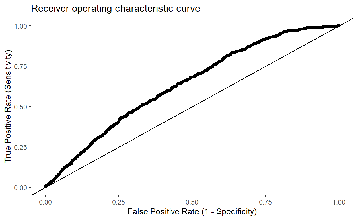
To estimate the area under the curve (AUC) we can just use the trapezium rule. (In fact we can be a bit lazy and not even do that, since the points are so close together.) The diff() function in R computes the differences between consecutive elements in a vector. If the function that describes the curve is \(y = f(x)\), then we want to compute \[\int_0^1 y~ dx \approx \sum_{i=1}^n y_i \cdot\Delta x_i,\] which can be achieved using the code:
similar to the estimate given by Stata.
Now recall the logistic regression model that used age as a categorical variable. Is this model adequate?
Again, we won’t use the Hosmer-Lemeshow test, but alternatives available in base R.
anova(model4, test = 'Chisq')
Analysis of Deviance Table

Model: binomial, link: logit

Response: hip_p == "yes"

Terms added sequentially (first to last)

         Df Deviance Resid. Df Resid. Dev  Pr(>Chi)
NULL                      4473     3378.1
agegroup  6  128.595      4467     3249.5 < 2.2e-16 ***
sex       1   32.753      4466     3216.8 1.046e-08 ***
---
Signif. codes:  0 '***' 0.001 '**' 0.01 '*' 0.05 '.' 0.1 ' ' 1
Yes, the model appears adequate.
What is the area under the ROC curve for this model?
      AUC
0.6498964
Create an age2 term and add this to the model with age as a continuous variable. Does adding this quadratic term improve the fit of the model?
Obviously it will improve the fit, but whether it is worth the added complexity is another question.
Call:
glm(formula = hip_p == "yes" ~ sex + age + I(age^2), family = binomial("logit"),
    data = epicourse)

Deviance Residuals:
    Min       1Q   Median       3Q      Max
-0.6809  -0.5912  -0.5124  -0.2951   3.1901

Coefficients:
              Estimate Std. Error z value Pr(>|z|)
(Intercept) -6.8154736  0.6747805 -10.100  < 2e-16 ***
sexM        -0.5499348  0.0932640  -5.897 3.71e-09 ***
age          0.1523200  0.0224885   6.773 1.26e-11 ***
I(age^2)    -0.0010601  0.0001827  -5.802 6.56e-09 ***
---
Signif. codes:  0 '***' 0.001 '**' 0.01 '*' 0.05 '.' 0.1 ' ' 1

(Dispersion parameter for binomial family taken to be 1)

    Null deviance: 3424.1  on 4514  degrees of freedom
Residual deviance: 3258.0  on 4511  degrees of freedom
AIC: 3266

Number of Fisher Scoring iterations: 6
Yes, the quadratic term appears to be significant.
Obtain the area under the ROC curve for this model. How does it compare for the previous models you considered?
Using the same procedure as above, we obtain the AUC:
      AUC
0.6469166
which is similar to the AUC for the model where age is a categorical predictor.
Diagnostics
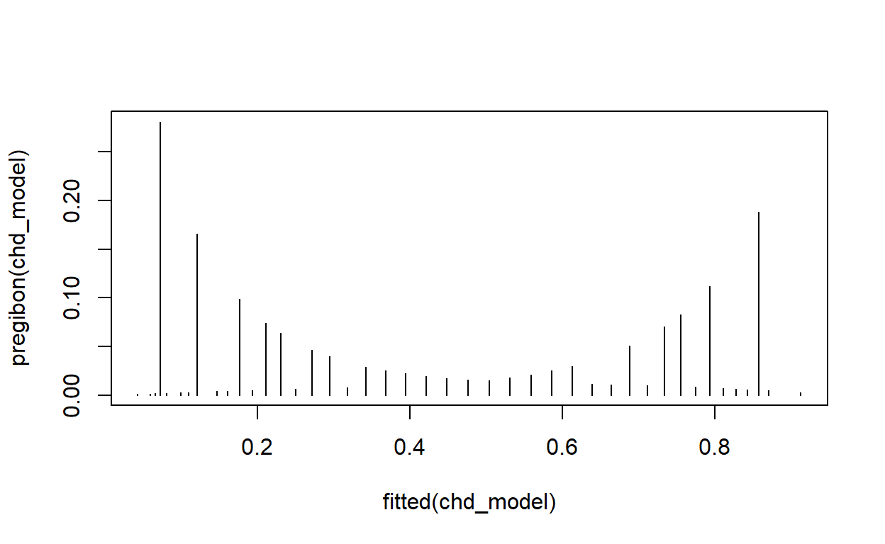
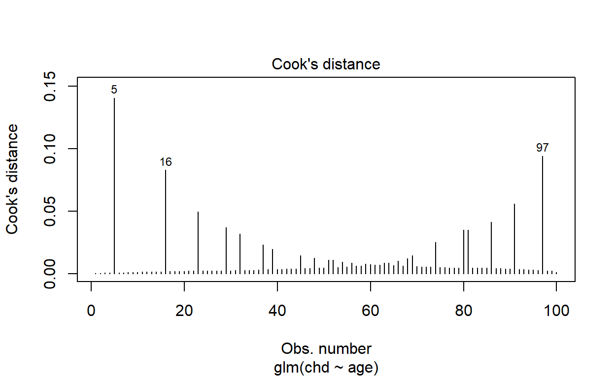
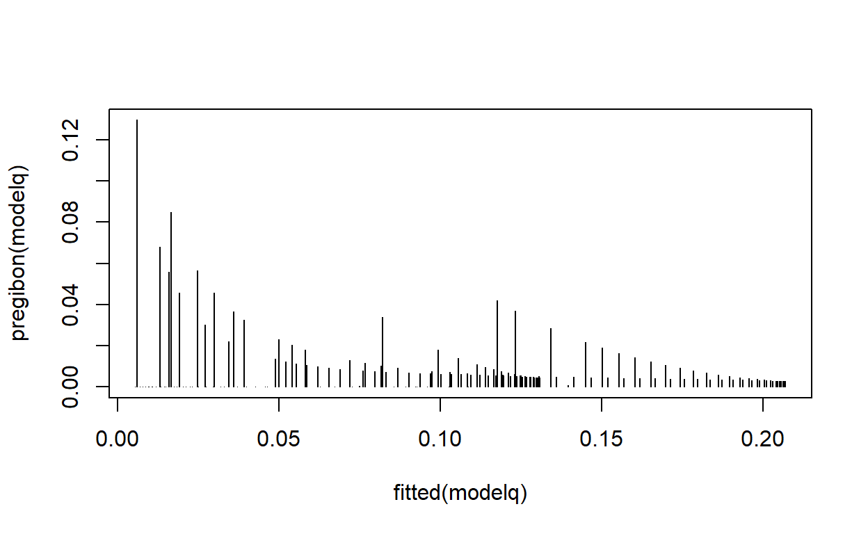
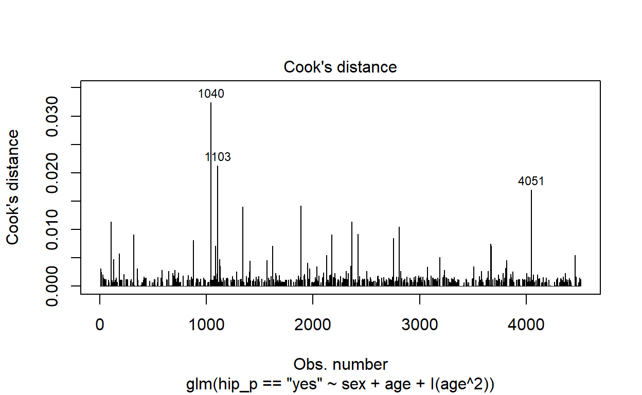
Produce a scatter plot of \(\Delta\hat\beta_i\) against fitted values for the previous regression model. Is there any evidence of an influential point?
Pregibon’s \(\Delta\hat\beta_i\) statistic, according to the Stata documentation, has the formula \[\Delta\hat\beta_i = \frac{r_j^2 h_j}{(1 - h_j)^2},\] where \(r_j\) is the Pearson residual for the \(j^\text{th}\) observation and \(h_j\) is the \(j^\text{th}\) diagonal element of the hat matrix.
It is not clear if there is an exact, named, equivalent in R, but we can try to compute it ourselves and then compare it with the other influence.measures() available.
pregibon <- function(model) {
  # This is very similar to Cook's distance
  r <- residuals(model, type = 'pearson')
  h <- hatvalues(model)
  r^2 * h / (1 - h)^2
}
plot(fitted(modelq), pregibon(modelq), type = 'h')
plot(modelq, which = 4)
Obtain the deviance residuals and plot them against the fitted values. Is there evidence of a poor fit for any particular range of predicted values?
Deviance residuals are accessible via residuals(model, type = 'deviance').
plot(fitted(modelq), residuals(modelq, type = 'deviance'),
     xlab = 'Fitted values', ylab = 'Deviance residuals')
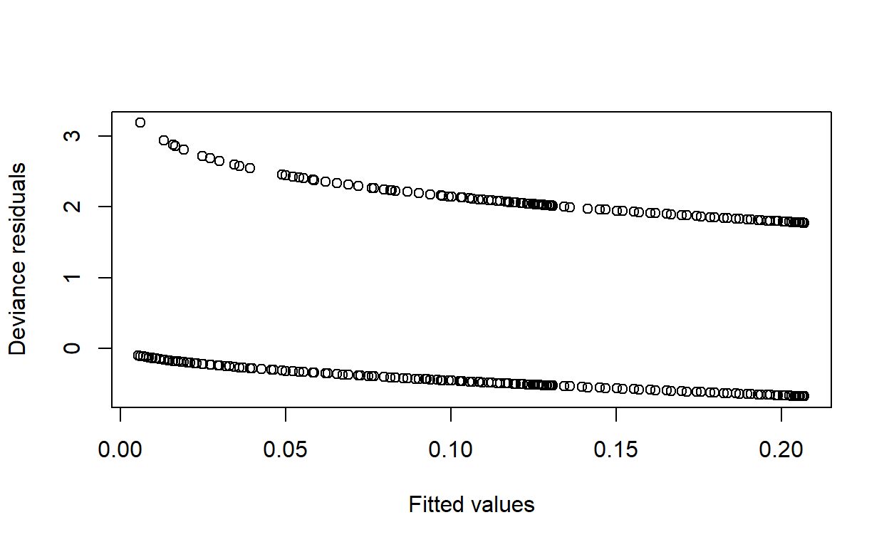
Again, this looks nothing like the plot in Mark’s solutions. Is there something wrong? It could be that the Stata version groups observations by “covariate pattern” and computes the influence based on all the points from the same pattern being removed, rather than simply leave-one-out. However, this is not clear.
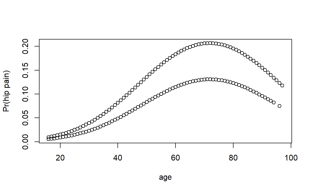
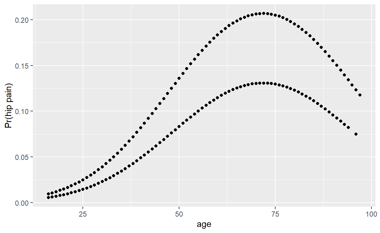
Plot fitted values against age. Why are there two curves?
Compare logistic regression model predictions to a non-parametric smoothed curve.
You can use loess(), or geom_smooth() in ggplot2. If you are having trouble, try adjusting the smoothing parameter (span), and make sure the variables are in a numeric/binary format, as loess() doesn’t really like factors.
ggplot(epicourse) +
  aes(age, as.numeric(hip_p) - 1) +
  geom_point(aes(y = fitted(modelq))) +
  geom_smooth(aes(colour = sex), method = 'loess', se = F, span = .75) +
  ylab('Pr(hip pain)')
nonpar <- loess(data = transform(epicourse,
                                 pain = as.numeric(hip_p == 'yes'),
                                 male = as.numeric(sex == 'M')),
                pain ~ age * male, span = .75)
plot(epicourse$age, fitted(modelq), xlab = 'Age', ylab = 'Pr(hip pain)')
lines(1:100, predict(nonpar, newdata = data.frame(age = 1:100, male = T)), col = 'steelblue')
lines(1:100, predict(nonpar, newdata = data.frame(age = 1:100, male = F)), col = 'tomato2')
legend('topleft', lty = 1, col = c('steelblue', 'tomato2'), legend = c('M', 'F'))
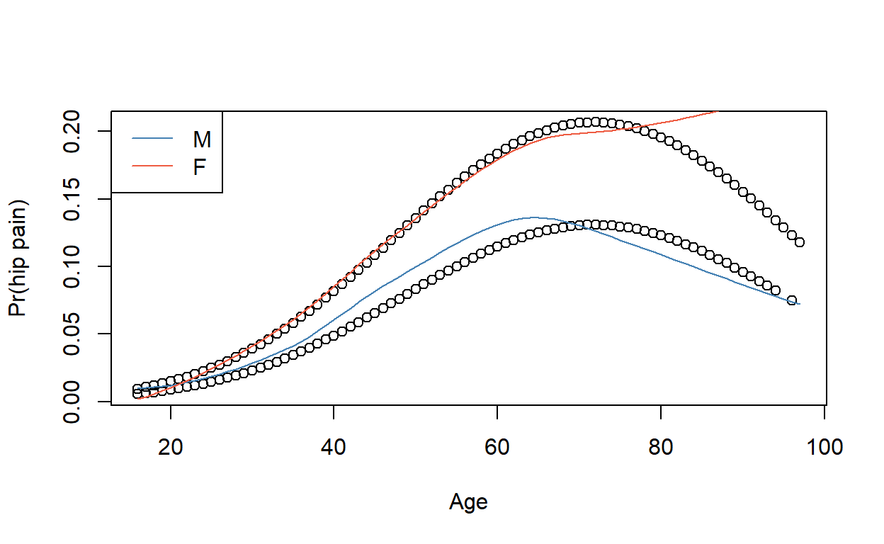
The quadratic model appears to fit fairly well for men, but not for elderly women.
The CHD data
This section of the practical gives you the opportunity to work through the CHD example that was used in the notes.
chd <- read.csv('chd.csv')
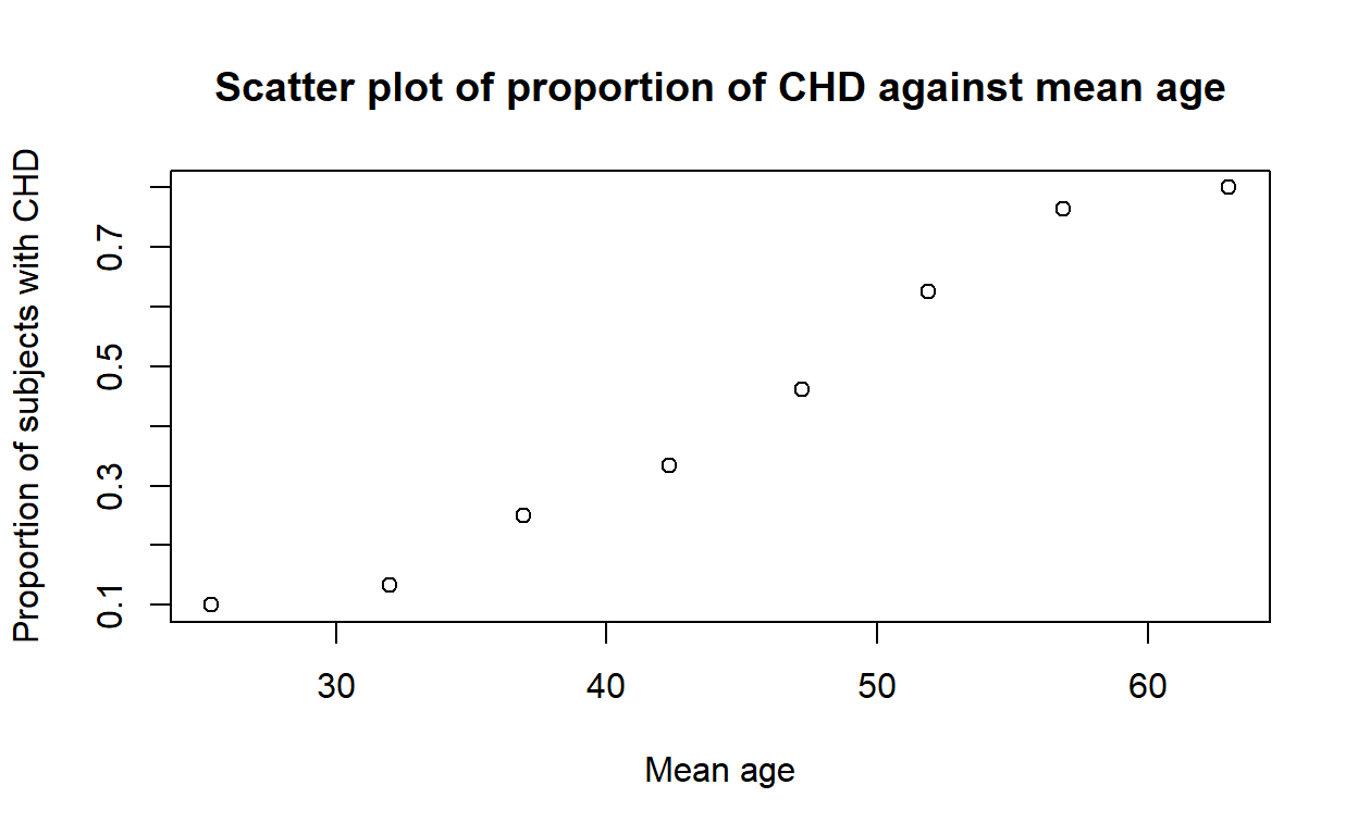
The following commands will reproduce Figure 1.2 using base R:
chd_means <- aggregate(cbind(age, chd) ~ agegrp, mean, data = chd)
plot(chd ~ age, data = chd_means,
     xlab = 'Mean age', ylab = 'Proportion of subjects with CHD',
     main = 'Scatter plot of proportion of CHD against mean age')
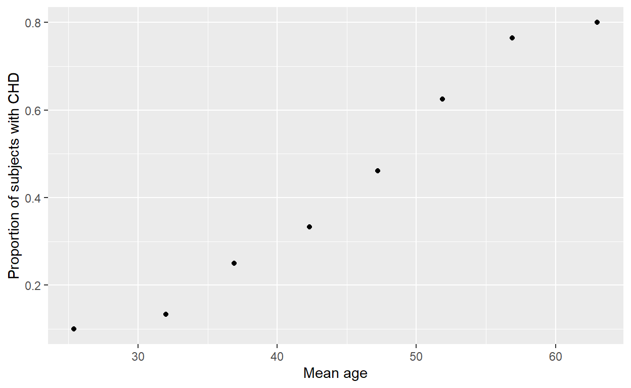
It can also be done in dplyr and ggplot2:
chd %>%
  group_by(agegrp) %>%
  summarise(agemean = mean(age),
            chdprop = mean(chd)) %>%
  ggplot() + aes(agemean, chdprop) +
  geom_point() +
  labs(x = 'Mean age', y = 'Proportion of subjects with CHD',
       main = 'Scatter plot of proportion of CHD against mean age')
Fit the basic logistic regression model with chd ~ age. What is the odds ratio for a 1 year increase in age?
Plot Pregibon’s \(\Delta\hat\beta_i\) against the fitted values for this model. Are any points particularly influential?