Tutorial on Transforming Hyperspectral Images to RGB Colour Images
This page provides an introduction to hyperspectral images and how hyperspectral reflectance or radiance image data can be transformed to RGB colour images.
A longer tutorial article on hyperspectral imaging in color vision
research is available on the JOSA website here or locally
here. See
also Spotlight
Summary.
1. Background
Hyperspectral images provide both spatial and spectral representations of scenes, materials, and sources of illumination. They differ from images obtained with a conventional RGB colour camera, which divides the light spectrum into broad overlapping red, green, and blue image slices that when combined seem realistic to the eye. By contrast, a hyperspectral camera effectively divides the spectrum into very many thin image slices, the actual number depending on the camera and application [1] [2]. This fine-grained slicing reveals spectral structure that may not be evident to the eye or to an RGB camera but which does become apparent in a range of visual and optical phenomena, including metamerism [3] and colour constancy [4].
To help understand its organisation, a hyperspectral image may be represented as a cube containing two spatial dimensions (pixels) and one spectral dimension (wavelength), as illustrated in Fig. 1. In this example (the original hyperspectral image is available here), the spectrum has been sampled at 10-nm intervals over 400-720 nm. At each sample wavelength, there is a complete intensity (grey-level) representation of the reflectance or radiance in the scene.
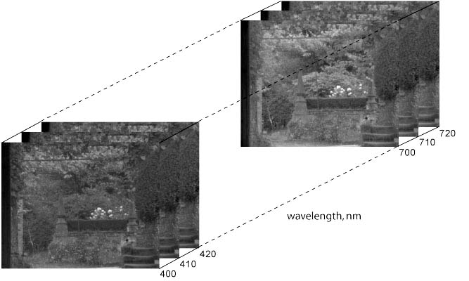 |
Figure 1. Hyperspectral image cube |
 |
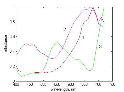 |
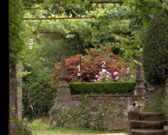
Figure 2. RGB scene image with three selected pixels |
Figure 3. Normalized reflectances at selected pixels of Fig. 2 |
Computations are performed in MATLAB (The MathWorks Inc.), which draws on the Matlab Image Processing Toolbox. Some supporting routines, data, and a small test hyperspectral image are also needed, all of which can be downloaded as a 15 MB zipped package here.
This package should be unzipped into a directory on the MATLAB path. Some familiarity with elementary MATLAB operations and basic colour science is assumed. For an introduction to both, see [5].
If you want to experiment with other hyperspectral images, then sets of reflectance files are available here and here and separate, larger sets of radiance files are available here and here. With some hyperspectral images, the edges may need trimming to remove pixels with zero or padded values that were introduced during postprocessing.
2. Contents of the package(download here)
ref4_scene4.mat is a test hyperspectral image consisting of an array of spectral reflectances of size 255 x 355 x 33. The first two coordinates represent spatial dimensions (pixels), in row-column format, and the third coordinate represents wavelength (400, 410, ..., 720 nm), as in Fig. 1. For ease of handling in this tutorial, the image has been reduced spatially to about a quarter of the size of those downloadable here.
illum_25000.mat, illum_6500.mat, and illum_4000.mat are three illuminant spectra, each vectors of length 33 (i.e. 400, 410, ..., 720 nm), representing the spectra of blue skylight with correlated colour temperature (CCT) 25000 K, daylight with CCT 6500 K, and evening sunlight with CCT 4000 K [6]. Formulae for generating daylight spectra are provided in [6].
xyzbar.mat
contains
the CIE 1931 colour-matching functions [6].
Tablulated values are also available here.
XYZ2sRGB_exgamma.m is a routine for converting tristimulus values XYZ to the default RGB colour space sRGB, but without gamma correction . A copy of the document IEC_61966-2-1.pdf explaining the full conversion of XYZ to sRGB is also included.
3. Reflectance data
Load
ref4_scene4.mat
and test the size of the resulting array reflectances.
load ref4_scene4.mat; |
It should
have size 255 x 335 x 33. To inspect reflectances,
try taking a slice at a
middle wavelength, say 560 nm (17th in the sequence 400, 410, , 720
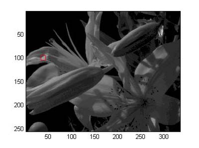
nm), and displaying it. The image should look like Fig. 4
(except for
the added red square, left).
slice = reflectances(:,:,17); |
 |
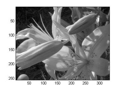 |
Figure 4. Slice from hyperspectral reflectance image at 560 nm |
Figure 5. As Fig. 4 with intensity levels clipped to level of red square in Fig. 4 |
brighten is used to compensate
roughly for the gamma of the monitor or display (i.e. the nonlinear
input-output function), and an equivalent effect can be produced with slice.^0.5,
or slice.^0.4, in place
of slice as the argument to imagesc.
The image still appears dark, however, because the exposure used during
image acquisition by the hyperspectral camera was determined by the
specular highlight at the top right of the scene. For presentational
purposes, therefore, the intensity levels of the image in Fig. 4 may be truncated by clipping to a level, z say, of a less-specular region
(all intensity levels above z
are then set equal to z), and
then rescaling. The clip level z
was taken from the pixel with row-column coordinates (100, 39) in the
red square. The image should now look like Fig. 5.
Detail in the darker areas is now much clearer than in Fig. 4.
z = max(slice(100, 39)); |
Now choose a different pixel in the scene, say with row-column coordinates (141, 75), and plot its spectral reflectance. The plot should look like Fig. 6.
reflectance =
squeeze(reflectances(141, 75,:)); |
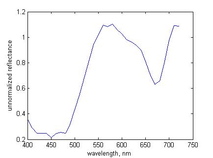 |
Figure 6. Unnormalized spectral reflectance at pixel (141, 75) |
reflectance
exceeds unity at some wavelengths, as in Fig. 6.
This is because the reflectances were normalized against an area on the
grey sphere at the bottom of the image, and the intensity of light
reflected from some other surfaces, at different angles, is
greater, e.g. at the pixel with row-column coordinates (100, 39).
The array reflectances may be normalized by
dividing by the maximum reflectance taken over all pixels and
wavelengths.
reflectances =
reflectances/max(reflectances(:)); |
For more a detailed explanation of normalization, see Section 6.2 later; also the technical notes section here and Appendix A of [3].
4. Radiance data
Load one of the illuminant spectra, say illum_25000.
Multiply each reflectance in the scene by this illuminant spectrum to
get the reflected radiances radiances_25000
(a for-loop is less efficient than MATLAB's bsxfun
function, but it makes little difference here). Using the same pixel as for Fig. 6,
plot the reflected radiant spectrum radiance_25000
(notice the different spelling). The spectrum should look
like curve 1 in Fig. 7.
load illum_25000.mat; |
Repeat with another illuminant spectrum, e.g. illum_4000.
The reflected radiance spectrum should look like curve 2 in Fig. 7. Notice how the
reflected spectra differ from each other and from the spectral
reflectance in Fig. 6.
load illum_4000.mat; |
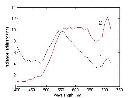 |
Figure 7. Reflected radiance spectra at pixel (141, 75) for illuminants with CCTs (1) 25000 K and (2) 4000 K |
5. Converting hyperspectral data to CIE XYZ and sRGB representations
Suppose you want to make an RGB representation of the scene in ref4_scene4.mat under a global
illuminant with CCT 6500 K. Load the
illuminant spectrum illum_6500 and obtain reflected
radiances radiances_6500.
load illum_6500.mat; |
For convenience, put radiances = radiances_6500.
The next step is to convert the radiance data radiances into
tristimulus values XYZ.
5.1. CIE XYZ image
Record the size of the array radiances,
and then reshape it as a matrix of w
columns for matrix multiplication with the colour-matching
functions. If you are working with an independent set of radiances,
e.g. from here
or here,
then just rename the hyperspectral image as radiances.
[r
c w] =
size(radiances); |
Load the CIE 1931 colour matching functions xyzbar and
take the matrix product of xyzbar with radiances
to get the tristimulus values XYZ at each pixel. For
simplicity XYZ is not normalized.
load xyzbar.mat; |
Correct the shape of XYZ so that it represents the
original 2-dimensional image with three planes (rather than a matrix
of 3 columns), and ensure that the values of XYZ
range within 0-1 (conventional normalization so that Y = 100 is
unnecessary here).
XYZ
= reshape(XYZ, r, c, 3); |
5.2. RGB colour image
To convert this XYZ representation of the image to the default RGB
colour representation sRGB (IEC_61966-2-1), excluding any gamma
correction, apply the transformation XYZ2sRGB_exgamma.
Ensure that the RGB values range within 0-1 by clipping
to 0 and 1 (or, if they greatly exceed 1, perhaps scaling by the
maximum).
RGB
= XYZ2sRGB_exgamma(XYZ); |
Finally, display the RGB image, including a rough gamma correction. The image should look like Fig. 8 (except for the added red square, bottom left).
figure;
imshow(RGB.^0.4, 'Border','tight'); |
|
|
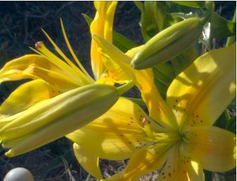 |
Figure 8. RGB image of reflected hyperspectral radiance image |
Figure 9. As Fig. 8 but intensity levels clipped to level of red square in Fig. 8 |
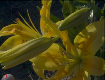
z
= max(RGB(244,17,:)); |
Nevertheless, clipping to the same value for all three RGB levels can lead to artifacts, and a more principled gamut-mapping procedure would preserve, for example, the hue and lightness of the clipped values [7].
Other examples of conversions from hyperspectral data to RGB images are available with reflectance files here and here and radiance files here and here.
6. Technical notes
Two issues need to be considered more carefully: one has to do with the non-smoothness of natural reflectance spectra and the other to do with effective spectral reflectance values. Further discussion can be found here or here.
6.1. Non-smoothness of natural reflectance spectra
Sample spectra from natural scenes recorded with a hyperspectral camera may appear less smooth than spectra from single pigments recorded with a spectroradiometer in the laboratory. The reason is that the physics of the two situations is very different. Natural scenes usually are complex, have non-uniform illumination, and are recorded remotely by the camera, whereas laboratory pigment spectra usually are simple, have uniform illumination, and are recorded with a non-imaging device that averages signals over large homogeneous areas of the specimen. Where imaging conditions coincide, hyperspectral imaging and spectroradiometric data can match closely (see e.g. spectra of acrylic paints imaged under laboratory illumination in Fig. 1 of [3]).
The complexity of natural spectra is due to several factors.
1. Many natural scenes contain foliage, and foliage contains pigments such as chlorophylls and carotenoids, and anthocyanins in autumn, which give multiple large and small absorbance peaks distributed over the visible spectrum (see e.g. [8]. Depending on the particular combination of these pigments, their presence can produce a variety of complex reflectance spectra from region to region.
2. There are important physical surface effects associated with reflection [9] [10], which cause the reflected spectrum to vary markedly across different microscopic areas. More generally, natural organic and inorganic materials are likely to be spatially nonuniform, and may be contaminated by dirt and moisture, which along with weathering and biological degredation contribute to the complexity of the recorded spectrum.
3. Natural illumination is often variegated. Direct illumination from the sun may be combined with indirect illumination from the sky, together with local nonlinear mutual illumination, transillumination, and occlusion. Time-lapse sequences of hyperspectral images of natural scenes showing changing patterns of illumination over the course of the day are available here, and described in [11]. Thirty hyperspectral radiance images of natural scenes with multiple embedded probe spheres showing variation in local illumination estimates are available here and described in [12].
4. A further complication with hyperspectral imaging of natural scenes comes from having to limit the camera exposure duration to avoid the effects of fluctuating illumination and movement within the scene. For a combination of reasons, the signal-to-noise ratio may be low at the extremes of the visible range. In particular, the transmittance of the tunable liquid crystal filter used in some hyperspectral imaging devices is poorest at short wavelengths, where the incident radiant power from the sun is also least. Image slices at 400 nm may be particularly noisy (see examples here and here). Images with higher signal-to-noise ratios, obtained by averaging spatially registered replicates, are available here, and described in [11].
Further discussion of natural spectra can be found in Section 3.C of [13].6.2. Effective reflectance values
The spectral reflectance of a surface element in a hyperspectral image is defined essentially as the quotient of the recorded radiant spectrum by the recorded radiant spectrum from a matt reference surface embedded in the scene, multiplied by the known spectral reflectance of the reference surface [3], Appendix A). From these effective spectral reflectance values, spectral radiance values can be recovered as outlined in Section 4.
Some of the spectral reflectance values available here and here exceed unity (also as in Fig. 6 here), despite the image being normalized with respect to a reference surface in the scene, usually a well-illuminated area (although see e.g. Fig. 2, bottom right). These excessive spectral reflectance values are a result of the optics of the scene and are intrinsic to these radiance calculations.
1. Excessive spectral reflectance values are due mainly to the nature of the bidirectional reflectance distribution function (BRDF) sampled by the scene and camera geometry. Thus when the reference surface is flat, it is almost always oriented with its surface normal towards the camera and away from the sun. But other surfaces in the scene may be oriented more favourably and be capable of reflecting more light to the camera. Even when the reference surface is spherical so that there is an optimal surface normal at some point (e.g. Fig. 8, bottom left), specular reflections from other surfaces in the scene may reflect more light to the camera (e.g. from water, as in Fig. 8, top right).
2. As explained in the technical notes section here, excessive spectral reflectance values are not important for a given scene and camera geometry, since it is the estimation of the reflected spectral radiance that matters. But for the analysis of the spectral reflectances themselves, it may be best to uniformly scale all the spectral reflectances in a hyperspectral image so that the greatest value does not exceed unity(Section 3, end). Unlike the manipulations for image presentation (Figs 5 and 9), spectral reflectances should not be scaled by ranked pixel values, e.g. the 90th or 99th centile, as this kind of clipping can substantially inflate both the spectral reflectance and accompanying noise estimates.
3. A fuller discussion of effective reflectances and effective illuminants is available in the technical notes section here, in Appendix A of [3], and in Sections 3.A and 3.B of [13].
4. A comparison of simulated global changes in illumination with
natural changes in illumination in which uneven changes in illumination
geometry were excluded at sample points is available in [11,
Sect. 3.6]. Depending on the sampling constraints, deviations in ratios
of cone excitations across pairs of sample points were 3.1%–4.8% with
simulated global changes in illumination spectrum and 3.1%–5.8% with
natural changes in illumination.
7. Hyperspectral imaging in color vision research
Reference [13] provides an introduction to terrestrial and close-range hyperspectral imaging and some of its uses in human color vision research. The main types of hyperspectral cameras are described together with procedures for image acquisition, postprocessing, and calibration for either radiance or reflectance data. Image transformations are defined for colorimetric representations, color rendering, and cone receptor and postreceptor coding. Several example applications are also presented. These include calculating the color properties of scenes, such as gamut volume and metamerism, and analyzing the utility of color in observer tasks, such as identifying surfaces under illuminant changes. The effects of noise and uncertainty are considered in both image acquisition and color vision applications.
If you use this material in published research, please cite the publication in full: Foster, D.H., & Amano, K. (2019). Hyperspectral imaging in color vision research: tutorial. Journal of the Optical Society of America A, 36, 606-627.8. References
- J. Y. Hardeberg, F. Schmitt, and H. Brettel, Multispectral color image capture using a liquid crystal tunable filter, Optical Engineering, vol. 41, pp. 2532-2548, 2002.
- H. F. Grahn and P. Geladi, Techniques and Applications of Hyperspectral Image Analysis, Chichester, England: John Wiley & Sons, Ltd, 2007.
- D. H. Foster, K. Amano, S. M. C. Nascimento, and M. J. Foster, Frequency of metamerism in natural scenes, Journal of the Optical Society of America A - Optics Image Science and Vision, vol. 23, pp. 2359-2372, 2006. [download PDF here]
- D. H. Foster, K. Amano, and S. M. C. Nascimento, Color constancy in natural scenes explained by global image statistics, Visual Neuroscience, vol. 23, pp. 341-349, 2006. [download PDF here]
- S. Westland and C. Ripamonti, Computational Colour Science using Matlab, Chichester, England: John Wiley & Sons, 2004.
- CIE, Colorimetry,
4th Edition, CIE Publication 015:2018 (CIE Central Bureau,
Vienna, 2018).
- J. Morovič, Color Gamut Mapping, Chichester, England: John Wiley & Sons, 2008.
- D. A. Sims and J. A. Gamon, Relationships between leaf pigment content and spectral reflectance across a wide range of species, leaf structures and developmental stages, Remote Sensing of Environment, vol. 81, pp. 337-354, 2002.
- J. B. Clark and G. R. Lister, Photosynthetic action spectra of trees. 2. Relationship of cuticle structure to visible and ultraviolet spectral properties of needles from 4 coniferous species, Plant Physiology, vol. 55, pp. 407-413, 1975.
- J. H. McClendon, The micro-optics of leaves. 1. Patterns of reflection from the epidermis, American Journal of Botany, vol. 71, pp. 1391-1397, 1984.
- Foster,
D.H., Amano, K., and Nascimento, S.M.C. (2016). Time-lapse ratios of
cone excitations in natural scenes. Vision Research, 120,
45-60,
http://dx.doi.org/10.1016/j.visres.2015.03.012. [download
PDF here]
- Nascimento,
S.M.C., Amano, K., and Foster, D.H. (2016). Spatial distributions of
local illumination color in natural scenes. Vision Research,
120,
39-44, http://dx.doi.org/10.1016/j.visres.2015.07.005. [download
PDF here]
- Foster, D.H. and Amano, K. (2019). Hyperspectral imaging in color vision research: tutorial. Journal of the Optical Society of America A, 36, 606-627. http://dx.doi.org/10.1364/JOSAA.36.000606. [download PDF here]
A Concise Guide to Communication in Science & Engineering
 |
|
|
| Published by Oxford University Press, November 2017, 408 pages. ISBN: 9780198704249. Available as hardback, paperback, or ebook. | ||