 |
Model-free estimation of a psychometric function |
|---|---|
| Home | Downloads | Demonstration | Documentation | Examples | Functions | Contacts |
|---|
Parametric fitting
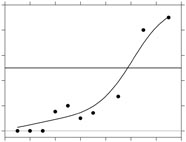
The psychometric function underlying a given set of data is traditionally fitted by assuming that it has a standard shape, e.g. a Gaussian or Weibull function, and adjusting its parameters for best fit. The correct model function, however, is rarely known, and as a consequence, the fit may be biased, leading to incorrect inferences.
In parametric fitting, a psychometric function P is estimated by a generalized linear model with binomial distribution. The model for the psychometric function consists of a link function l (ensuring the response does not take impossible values) and a linear function of the stimulus levels x. The link function transforms the psychometric function to a linear function η; that is l(P(x)) = η = a0 + a1 x. Equivalently, P(x) = l –1(a0 + a1 x). The link l is specified a priori, and it is defined by the chosen model function and the specified guessing and lapsing rates. For example, if the chosen model function is Gaussian and both guessing and lapsing rates are assumed to be zero, then the link function is simply the inverse of the Gaussian cumulative distribution function (see McCullagh and Nelder (1989), and Żychaluk and Foster (2009) Download PDF). The parameters a0 and a1 are estimated by maximizing the log-likelihood,
l(a0, a1) = ∑i[ki ln(P(xi)) + (mi – ki) ln(1 – P(xi))].
The fit is strongly dependent on the chosen link function. The correct link function, however, is rarely known, and as a consequence, the fit may be biased, leading to incorrect inferences.
Local linear fitting
To avoid these problems, the psychometric function can be modelled locally. The link function is still needed to ensure that the psychometric function does not take prohibited values but the function after transformation is no longer assumed to be linear. The only assumption is that it is smooth. By a Taylor expansion, any smooth function can be approximated locally by a linear function
l(P(xi)) = η ≈ a0 + a1 (xi – x),
where the parameters α0, α1 depend on x and their values are estimated by maximizing local log-likelihood,
l(x) = ∑i[ki ln(P(xi)) + (mi – ki) ln(1 – P(xi))] w(x,xi).
The weights w(x,xi) determine the influence of each point xi on the estimate at a point x: the further the points x and xi are apart, the smaller the value of w(x,xi).
The weight funciton is defined as w(x,xi) = K((x – xi)/h)/h for a kernel K and a bandwidth h. The kernel is a function usually assumed to be positive and symmetric about zero, e.g. a Gaussian function. It is known that the influence of the weight function w depends less on the shape of the kernel K than on the bandwidth h. The choice is crucial, as h controls the domain of influence of w and hence the smoothness of the local linear estimate. For small h, the estimate follows the data very closely and is therefore susceptible to the random variations in the data. For large h, the estimate is very smooth, close to that obtained by a parametric method, and therefore potentially biased.
To decide what is an optimal bandwidth, first the appropriate loss function needs to be chosen. This is a function which measures discrepancy between the true psychometric function and the estimate. The most commonly used measures are deviance (McCullagh and Nelder (1989), Żychaluk and Foster (2009) Download PDF) and integrated squared error (ISE),
ISE(ĝ) = ∫ (g(x) – ĝ(x))2 dx,
where g is the function of interest and ĝ the estimator of this function. Here, the ISE was considered both for the psychometric function P and for the function η. Thus there are three possible loss functions: the deviance, ISE for the psychometric function P, and ISE for the function η. There are also three main methods of bandwidth choice available in this package: the plug-in, cross-validation, and bootstrap. The plug-in bandwidth estimates the ISE-optimal bandwidth for the function η. For cross-validation and bootstrap, there are three possible loss functions as just described.
Finally, once the data have been fitted, there are several ways to assess the goodness of fit, such as the deviance or Pearson's X2. With psychometric functions, the responses are binomially distributed, but if they were normally distributed, then the deviance would coincide with the residual sum of squares.
Reference: McCullagh, P. and Nelder, J. A. Generalized linear models, 1989, London: Chapman & Hall.
A how-to guide to finding nonparametric estimates of psychometric functions with this package (MatLab option) follows.
The data in a text file should be in three columns, with no header: first column for stimulus levels, second for number of successes, and third for number of trials. Each line in the file should correspond to a stimulus level and the values should be separated by spaces. An example follows
0.1 0 3
0.2 0 3
0.3 0 5
0.4 2 13
0.5 2
				10
0.6 2 20
0.7 2 14
0.9 3 11
1.1 4 5
1.3 18 20
To load the data in MatLab write
[ x, r, m ] = textread( '<path\filename>' );
To save the loaded data in MatLab format, type
save('<path\filename>', 'x', 'r', 'm');The
filenameshould have extension ".mat" or no extension. Once created it can be loaded by typing
load('<path\filename>');
Local linear fitting is performed by the function
locglmfit. The arguments arexfit– points in which the function is to be estimated,r– the number of successful responses,m– the number of trials,x– stimulus levels, andbwd– bandwidth. The syntax is
pfit = locglmfit( xfit, r, m, x, bwd );
The selection of bandwidth is critical in local linear fitting. In this package there are three functions to select the bandwidth,
bandwidth_bootstrap,bandwidth_cross_validation, andbandwidth_plugin. For all the methods, the number of successesrinmtrials at each stimulus levelxare mandatory parameters.For the function
bandwidth_bootstrapa search intervalbwdIntervalfor the optimal bandwidth and the number of bootstrap replications are also mandatory. The syntax is
bwd = bandwidth_bootstrap( r, m, x, bwdInterval, replications );For the function
bandwidth_cross_validationa search intervalbwdIntervalfor the optimal bandwidth is also mandatory. The syntax is
bwd = bandwidth_cross_validation( r, m, x, bwdInterval );The function
bandwidth_plugincalculates an estimate of the AMISE optimal bandwidth for the local polynomial estimator of a psychometric function. The syntax is
bwd = bandwidth_plugin( r, m, x);An additional function, used only for testing purposes, is the function
bandwidth_optimal. This function finds the actual optimal bandwidth for synthetic data with known, true psychometric functionptrue. The arguments for this function are the same as forbandwidth_cross_validation, except that the true psychometric functionptrueis also required. The syntax is
bwd = bandwidth_optimal( ptrue, r, m, x, bwdInterval );
Calculates deviance
Dfor data and fitted values of the psychometric functionpfit. The syntax is
D = deviance( r, m, pfit );
The package also provides fits for several parametric models, such as Gaussian, Weibull, reverse Weibull, and logistic cumulative distribution functions. The parameters are estimated in functions
binomfit_lims,binom_weib, andbinom_revweib. The fitted values are obtained with the functionbinomval_lims.To fit a logistic function and calculate the fitted values, the syntax is
b = binomfit_lims( r, m, x );

                fest = binomval_lims( b, xfit );
To fit other functions, e.g. the Gaussian cumulative distribution, check the optional inputs of the function
binomfit_lims.To fit a Weibull function, the optimal exponent
Kfor the Weibull needs to be estimated in addition to the linear coefficientsb. To obtain the estimated psychometric function at valuesxfit, the guessing and lapsing rate (in this example both are equal to0) and the estimated power parameterKneed to be provided inbinomval_lims. The syntax is
[ b, K ] = binom_weib( r, m, x );

                fest = binomval_lims( b, xfit, 'weibull', 0, 0, K );
To fit a reverse Weibull function and calculate the fitted values, replace the function
binom_weibbybinom_revweibin the previous code and the parameter'weibull'by'revweibull'in the functionbinomval_lims.
The link functions available in the package are
- logit
- probit
- loglog
- comploglog
- weibull
- revweibull
The kernels available in the package are
- normpdf
- epanechikov
- triangular
- tricube
- bisquare
- uniform
The loss functions available to estimate the optimal bandwidth by
bandwidth_bootstrap,bandwidth_cross_validation, orbandwidth_optimalare
- ISE: Integrated squared error
- ISEeta: Integrated squared error on eta scale(eta is the function that is related to the psychometric function via the link function)
- deviance function
Check the Functions to see how to modify both links and kernels in the different functions.