MATLAB Short Course 2: Symbolic manipulation, graphics
Contents
Define the symbolic variables
syms x
syms y z
limit, integration, differentiation
limit((1-cos(x))/x^2,x,0)

int(1/sqrt(1+x^2),x)

diff(1/sqrt(1+x^2),x)

diff(1/sqrt(1+x^2),x,2)  % last 2 means taking derivatives twice

diff(1/sqrt(1+x^2),x,3)
ans =

1/2


ans =

asinh(x)


ans =

-x/(x^2 + 1)^(3/2)


ans =

(3*x^2)/(x^2 + 1)^(5/2) - 1/(x^2 + 1)^(3/2)


ans =

(9*x)/(x^2 + 1)^(5/2) - (15*x^3)/(x^2 + 1)^(7/2)
Taylor expansion
taylor(cos(x),x,0)
taylor(cos(x),x,0,'Order',10)
ans =

x^4/24 - x^2/2 + 1


ans =

x^8/40320 - x^6/720 + x^4/24 - x^2/2 + 1
solve polynomial equations
syms x p q
solve(x^2+p*x+q==0,x)  % notice the double equal sign "=="
ans =

- p/2 - (p^2 - 4*q)^(1/2)/2
  (p^2 - 4*q)^(1/2)/2 - p/2
the result may not always what you expect
roots of the cubic equation
syms p q x
solve(x^3+p*x+q==0,x)
ans =

root(z^3 + p*z + q, z, 1)
root(z^3 + p*z + q, z, 2)
root(z^3 + p*z + q, z, 3)
get numbers from symbolic solutions via "double"
solve(x^3+x+1==0,x)
double(ans)     % ans is the last (named or un-named) result
ans =

root(z^3 + z + 1, z, 1)
root(z^3 + z + 1, z, 2)
root(z^3 + z + 1, z, 3)


ans =

  -0.6823 + 0.0000i
   0.3412 - 1.1615i
   0.3412 + 1.1615i
symbolic sum/product
syms k n
symsum(k,k,1,n)
symsum(1/n^2,n,1,inf)
symprod((n^2-1)/n^2,n,2,inf)
ans =

(n*(n + 1))/2


ans =

pi^2/6


ans =

1/2
MATLAB plot
the key is to generate the data points
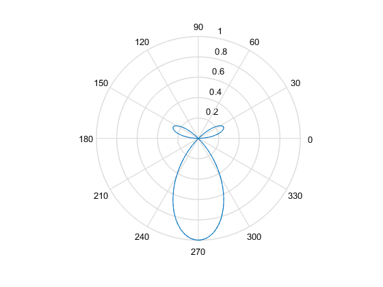
x = -10:0.1:10;
y = sin(x);
plot(x,y)

% change the plot style
plot(x,y,'*')
plot(x,y,'-*')

% polar plot
t = linspace(0,2*pi,100); % same as:  t = 0:0.01:2*pi;
rho = sin(t).*cos(2*t);   % note the use of "." pointwise product
polar(t,rho)
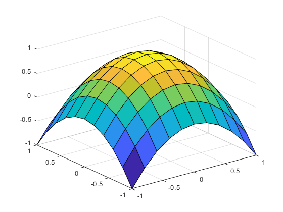
plot surfaces
x = linspace(-1,1,11);
y = x;
[X, Y] = meshgrid(x,y);  % have a look at both X and Y
Z = 1-X.^2-Y.^2;
surf(x,y,Z)
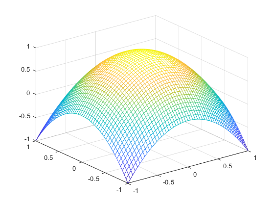
surface on a denser mesh
x = linspace(-1,1,51);
y = x;
[X, Y] = meshgrid(x,y);
Z = 1-X.^2-Y.^2;
mesh(x,y,Z)  % or surf(x,y,Z)
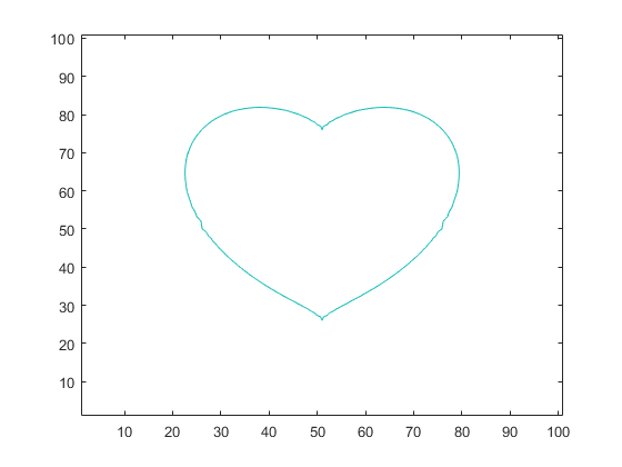
Contour for the heart shaped curve
x = linspace(-2,2,101);
y = x;
[X, Y] = meshgrid(x,y);
Z = (X.^2+Y.^2-1).^3-X.^2.*Y.^3;
contour(Z,[0 0])