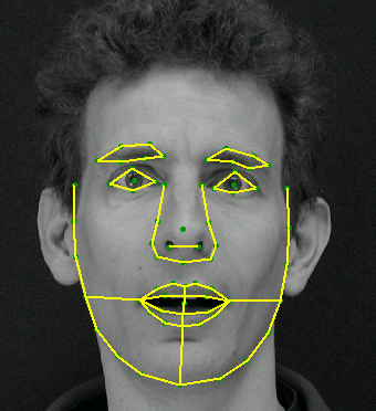
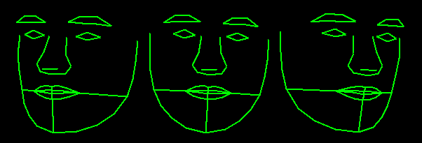
The first mode of shape variation of a training set containing many different view points tends to represent rotation of the head.
Given a set of examples of a shape, we can build a statistical shape model. Each shape in the training set is represented by a set of n labelled landmark points, which must be consistant from one shape to the next. For instance, on a hand example, the 7th point may always correspond to the tip of the thumb.
Given a set of such labelled training examples, we align them into a common co-ordinate frame using Procrustes Analysis. This translates, rotates and scales each training shape so as to minimise the sum of squared distances to the mean of the set.
Each shape can then be represented by a 2n element vector
x = (x_1, ... , x_n, y_1, ... , y_n).
The aligned training set forms a cloud in the 2n dimensional space, and can be considered to be a sample from a probability density function.
In the simplest formulation, we approximate the cloud with a gaussian.We use Principal Component Analysis (PCA) to pick out the main axes of the cloud, and model only the first few, which account for the majority of the variation.
The shape model is thenx = x_mean + Pb
where x_mean is the mean of the aligned training examples, P is a 2n x t matrix whose columns are unit vectors along the principal axes of the cloud, and b is a t element vector of shape parameters.
(This model has been dubbed a "Point Distribution Model" (PDM), but has little to do with the Point Distribution in statistics)
By varying the shape parameters within limits learnt from the training set, we can generate new examples.
Such models are used in the Active Shape Model framework to locate new examples in new images.
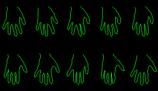
Consider the outline of a hand, represented by 72 labelled points.
Here are some examples from a training set:
By varying the first three parameters of the shape vector, b, one at a time, we can demonstrate some of the modes of variation allowed by the model:
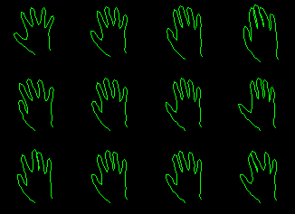
(Each row obtained by varying on parameter and fixing others at zero)
Here represent the shape of the facial structures with 68 points

The first mode of shape variation of a training set containing many different
view points tends to represent rotation of the head.

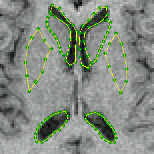
We can represent the outline of several brain structures in a single model.
For instance, here is an example from a labelled brain MR image
By varying the first two parameters of the shape vector, b, one at
a time, we can demonstrate some of the modes of variation allowed by the model:
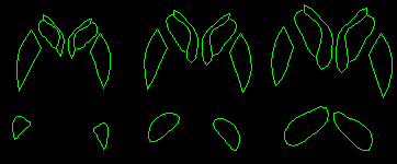
Varying the most significant parameter.
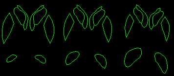
Varying the second most significant parameter.
You can now download a set of tools to build and play with Appearance Models and AAMs here. Enjoy.
Tim Cootes