The DOSY Toolbox
Mathias Nilsson and Gareth A. Morris.
School of Chemistry, University of Manchester, Oxford Road, Manchester M13 9PL, UK.
Version 0.53 – 15 March 2008
The current release is a beta version and should be obtained directly from Mathias Nilsson, University of Manchester (mathias.nilsson@manchester.ac.uk).
Although it is distributed under the GNU General Public License (see below), I would be grateful if users would not copy the code to others for the time being; this is so that I can keep track of users, versions and feedback. Once beta testing is complete I intend to allow unrestricted copying.
Dr. Mathias Nilsson
School of Chemistry, University of Manchester,
Oxford Road, Manchester M13 9PL, UK
Telephone: +44 (0) 161 275 4668
Fax: +44 (0)161 275 4598
mathias.nilsson@manchester.ac.uk
Contents
Quick start
Chances are that you probably don’t want to read all the manual but just get started processing. Assuming you have some experience in processing NMR data, this is for you!
- Install the software (I am afraid that you may have to read the instructions for that).
- Start the programme by clicking on the icon (for the MATLAB® version just type “DOSYToolbox“ in your MATLAB prompt).
- Import a data set using the “file” menu.
- Pre-process your raw NMR data, using the panels, before DOSY analysis. You will recognise many standard features in the panels such as phasing, zero filling, referencing and baseline correction.
- Choose one of the methods in the “Advanced Processing” panel; set your parameters and click “run” to start the processing.
- Inspect the result in the resulting DOSY or component spectra.
All the screenshots for the Quick start uses the data set “GUI_testdata_fiddled.fid”. This data set is from a mixture of quinine, geraniol and camphene in methanol-d4 with TSP as a reference material, measured on a Varian 400 MHz Inova spectrometer.
The data set has been reference deconvoluted and saved as such in the Varian Vnmr6.1C software. The raw data is also available as “GUI_testdata_raw.fid”.
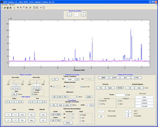
Main processing window
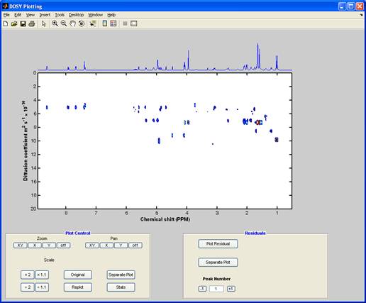
DOSY plot (output from the “DOSY” processing)
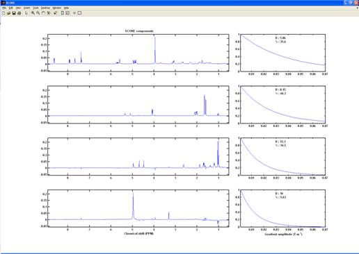
SCORE components (output from the “SCORE” processing)
Introduction
The importance of high resolution PFGNMR data for mixture analysis is steadily increasing, but there is no single best way to process such data. The commonest family of processing methods is known as DOSY (diffusion-ordered spectroscopy), and therefore it has become customary to refer to these data as DOSY data. The major NMR manufacturers each offer different limited implementations of DOSY processing in their current software. The DOSY Toolbox is a free programme that allows users of all three instrument families access to the same wide range of processing schemes.
The DOSY Toolbox has a graphical user interface for easy access to the main processing schemes (a small number of specialised features are only available from the command line in the MATLAB® version). It is written in MATLAB, but is also available as free-standing compiled version that does not require any MATLAB installation. The MATLAB version runs on any platform, the compiled version is presently only available under Windows.
Basic features
These are common for most high resolution NMR:
Window functions, phasing, baseline correction and referencing
Reference deconvolution
Import of raw data from Varian, Bruker and JEOL data
Diffusion processing
High Resolution DOSY1, 2. (This is what is most commonly referred to as DOSY)
Multiexponential DOSY3
DECRA4-6
MCR7, 8
SCORE9
All of the above methods can be corrected for the non-uniformity of the pulsed field gradients, but this requires careful calibration1, 3, 5, 9-11
The MATLAB version should run on any platform with MATLAB version 7.0 or greater. It is presently dependent on the Optimization and Statistics Toolboxes. The dependence on the Statistics Toolbox is minor and will be removed in future releases (presently it is needed for multiexponential fitting in DOSY and to use PCA-Varimax for starting values in MCR-ALS).
The free-standing version is currently limited to the Windows platform, but contains the vast majority of the important features of the MATLAB version.
Installation
The installation is dependent on the version you have received (MATLAB or free-standing).
MATLAB version
This is a set of m-files that should work with MATLAB v7.0 or higher on any platform. In addition to basic MATLAB it is also dependent on the Optimization and Statistics Toolbox
1. Unzip the DOSYToolbox_vXXX.zip to your preferred directory.
2. Add that directory (with subdirectories) to the MATLAB path.
3. Type “DOSYToolbox” to start the graphical user interface.
Free-standing version
This is dependent on the MATLAB Component Runtime (MCR) library, which I can normally provide with the DOSYToolbox software. A different version of the MCR library is needed for each platform and for each version of the MATLAB compiler used to generate the free-standing code. If the DOSYToolbox does not run as expected you may be using the wrong MCR library; please contact me for an updated version. The MCR library only needs to be installed once on each machine, and not for subsequent versions of the DOSYToolbox provided these used the same version of the MATLAB compiler. Please note that the MCR is about 120 Mb so it cannot easily be distributed by email but should in the future be included in the version of the DOSY toolbox downloadable from my homepage (http://personalpages.manchester.ac.uk/staff/mathias.nilsson/)
1. Only for the first installation of the programme.
You may require to install Microsoft Visual C++ 2005 SP1 Redistributable Package (x86). (http://www.microsoft.com/downloads/details.aspx?familyid=200b2fd9-ae1a-4a14-984d-389c36f85647&displaylang=en.)
2. Only for the first installation of the programme.
You will need first to install the version from my homepage (DOSYToolbox_v04_pkg.exe). Put the installer in your preferred directory and run it. This will install an early version of the programme together with the MCR libraries (you may want to remove the MCRInstaller.exe afterwards – see next step).
http://personalpages.manchester.ac.uk/staff/mathias.nilsson/
3. Installation of an update.
The program is distributed in the file DOSYToolbox_pkg_vXX_uppdateXXX.ex_. First rename the programme to DOSYToolbox_pkg_vXX_uppdateXXX.exe (it is just renamed to try and fool some simple firewalls, so that I can more easily distribute it via email). To install the programme, copy the file to your preferred directory and run it. However, if the MCRInstaller.exe is present in that folder it will be automatically run, so it may be useful to remove MCRInstaller.exe after the first installation.
4. Start the programme by clicking on DOSYToolbox.exe
The graphical user interface
When you start the DOSYToolbox, the main window will open, which provides access to (almost) all processing capabilities via processing panels and menus:
Menus
Files menu
The files menu contains ways to import, save and export data files (the structure of the DOSYToolbox files is described in Appendix A).
Open:
Opens data files saved by the DOSYToolbox (*.nmr)[a].
Import:
Imports raw data files (FIDs) from the main NMR manufacturers[b].
Save:
Saves the current data as *.nmr (see footnote for Open).
Export:
Different formats for exporting your data.
1. DOSY Processing:
Exports the data as *.pfg.; this is the standard MATLAB (*.mat) format and can be imported into MATLAB using “load –mat filemname.pfg” and will contain the data in a MATLAB structure of the form required by the command line processing functions: decra_mn, dosy_mn, mcr_mn and score_mn.
Edit menu
Parameters
This gives access to the diffusion-dependent parameters. Only when known standard pulse sequences have been used for acquisition can these be correctly imported, otherwise they have to be entered by the user
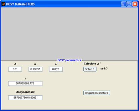
The parameters are :
Δ: diffusion time
Δ′: corrected diffusion time
δ: total pulse width for the diffusion encoding pulse field gradient
dosyconstant: γ2× δ2 × Δ′
γ: magnetogyric ratio of the nucleus (normally 1H)
The parameter “dosyconstant” is what is actually used in the calculations, and it can be entered manually. Changing either of the other parameters will prompt you to calculate the dosyconstant using one of the options (presently only one). NEED TO ADD TAU FOR BPP
Processing sections
These sections contain the tools to process the imported DOSY data.
Spectrum number:
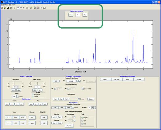
This panel is used to flick through the spectra, or FIDs, for the different gradient levels.
Phase correction
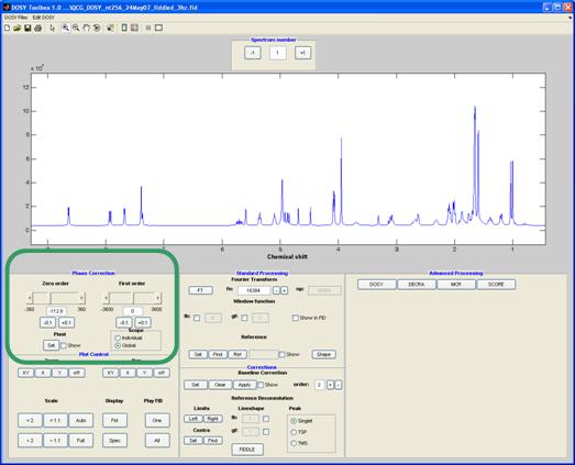
Zero and first (linear) order phase correction is applied using the side bars. Pressing the set button enables you to set the pivot point at which the first order correction is zero. Clicking the slider itself adjusts the phase in steps of 10 (degrees), the arrows on the slider in steps of 1 and the buttons below in steps of 0.1. An exact number can also be entered in the display box.
The phase correction can have two different modes. When the scope is set to global (default) the same phase correction is applied to all the spectra in the array; when a phase correction is needed for each spectrum in the array the scope is set to individual and each array element is phased individually. The individual mode allows the common problem of a gradient dependent zero order phase to be corrected.
Plot control
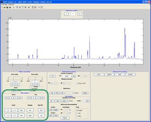
This panel allows the user to zoom, expand, auto scale the spectra and the FIDs. If you (not) are musically inclined you can also listen to the FIDs.
Standard processing
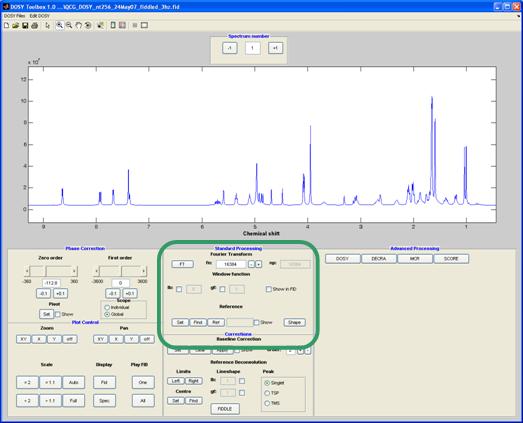
In this section you will find many tools to preprocess the data before performing more advanced (i.e. DOSY) processing.
Fourier Transform
Here you set the number of points used for the Fourier transform; default is the number of FID points.
Window function
Any window function will be multiplied with the FID before Fourier transformation. These can be exponential, Gaussian or a combination of the two. The exponential function Fourier transforms to a Lorentzian shape with the peak width at half height determined by(Lw) Lorenzian width (in Hz) , is as stated in:
![]()
The Gaussian function Fourier transforms to a Gaussian shape with the peak width at half height determined by (Gw) Gaussian width (in Hz) , is as stated in:
![]()
![]()
![]()
The window function can be visualised in the FID by clicking the check box.
Reference
The spectrum can be referenced to a reference line which is set with the “set” button. When clicking the “find” button an attempt to find the maximum of the nearest peak is done.
The shape button gives you the peak width at half height for the selected peak.
Corrections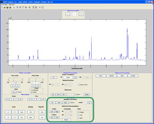
In this panel correction of the data can be applied before further processing.
Baseline correction
This requires that the regions of clear baseline in the spectrum be identified, by marking up all the signal-containing regions. After clicking the "set" button, each click of the mouse in the spectrum marks a point at which baseline changes to signal or vice versa. Each area of signal is marked with a green line; when the spectrum is ready for correction (using the "apply" button), all the signal areas show a green line. The baseline is corrected by fitting the baseline regions (those areas not marked by a green line) to a polynomial of the order specified.
Reference deconvolution
Reference deconvolution12, 13 attempts to correct for systematic errors in the data using the difference between the experimental and perfect shape of a known signal; this signal should be a well separated singlet.
Under “Limits”, click the “left” and “right” buttons to set the limits of the reference signal – this should include some pure baseline on each side. The “centre” button sets the centre frequency of the signal. The target lineshape is set using the lb and gf values (see Window functions) under “Lineshape”. Clicking the “FIDDLE” button applies the reference deconvolution; the type of reference peak is set to either singlet, TSP or TMS.
To undo the reference deconvolution, simply Fourier transform the data again.
Advanced processing
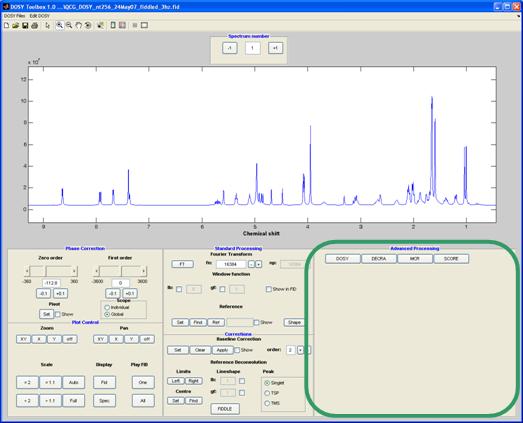
In this panel, the method to be applied to the (now pre-processed) data is selected by pressing the corresponding button. Each button displays a set of relevant parameters. All methods have the following common features:
Process – run the method with the current setting
Replot – replot the last data obtained with the current method
Exclude regions – regions that are not of interest (e.g. solvent peaks) can be selected in the same manner as for baseline correction. These regions will be excluded from analysis,
Prune – a space delimited list of gradient level numbers to be excluded from analysis. NB. This is likely to violate to the assumptions of DECRA processing.
Some information on the respective processing method can be found below. More information can be found in the MATLAB m-files for the respective processing method (dosy_mn.m, decra_mn.m, mcr_mn.m and score_mn.m).
DOSY

The DOSY button gives access to both the (standard) high resolution DOSY2 and multiexponential fitting3. In DOSY the decay of each individual peak-amplitude as a function of pulsed field gradient strength is fitted to the theoretical expression. The 2D DOSY plot is constructed using Gaussian peaks in the diffusion dimension centred on the fitted value and the width determined by the statistics of the fit.
Method-specific controls:
Thresh – set threshold below which all data will be excluded from analysis
Peak pick – use peak picking or fit each data point individually
Fit method – Fit to the (standard) exponential decay or use an equation corrected for non-uniformity of the field gradients (NUG)[c].
NUG coeff – coefficients for the NUG correction1, 3, 5, 9-11, 14[d]
Max ncom – maximum number of components (exponentials) per peak[e]. Default is 1 (HR-DOSY).
Tries per peak - number of different random starting values tested for a multiexponential fit
Min D – the smallest diffusion coefficient ( × 10-10) displayed in the DOSY plot
Max D – the largest diffusion coefficient ( × 10-10) displayed in the DOSY plot
D resolution – number of data points calculated in the diffusion dimension
DECRA
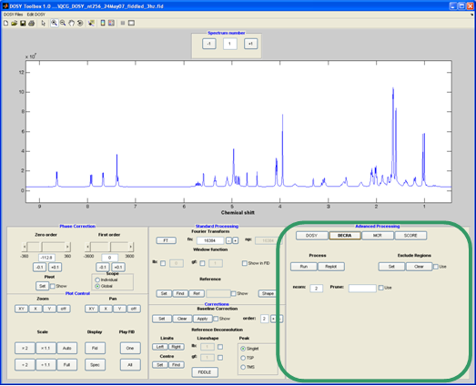
Direct Exponential Curve Resolution Algorithm (DECRA4, 6) attempts to decompose the DOSY data into a set number (“ncom”) of spectra and decays. DECRA is very fast but to give correct results the data need to conform to certain assumptions. One of the most important is that the diffusion decays are pure exponential (Stejskal-Tanner equation). This means that data must be sampled with equal spacing in gradient squared (don’t try to do a DECRA fit if the data are linearly spaced). It also means that DECRA is prone to artefacts when the gradients are not uniform, but this can be partly solved by using slice selection for acquisition or by tweaking the gradient levels5.
Method-specific controls:
ncom: the (user-) estimated number of components present in the mixture
MCR

Multivariate Curve Resolution is an umbrella name of a number of methods. Here a simple form of MCR-ALS (alternating least squares) is implemented7, 8, 15-18. Initial guesses can be made either as “spectra” or “decays”. The initialisation method can be either PCA-VARIMAX or DECRA (note that you need to have the gradient levels equally spaced in gradient squared, for the latter).
During the ALS loop certain constraints can be applied to the data. These includes non-negativity for the decays and/or for the spectra. In addition, the decays can be forced to follow either the Stejskal-Tanner (pure exponential) or the NUG function (see DOSY above).
Method-specific controls:
ncom: the (user) estimated number of components present in the mixture
Init Guess: Start with initial estimates of spectra or decays
Init Method: Method for estimating initial spectra (command line use of mcr_mn allows the usage of any user-supplied spectra or decays)
Dec constr: constraints for the decays
Spec constr : constraints for the spectra
Force decay: the decay is forced to a predetermined shape (exponential or NUG)
SCORE
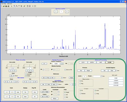
Speedy Component Resolution (SCORE)9 estimates the spectra assuming a predetermined shape of decay (exponential or NUG).
Method-specific controls:
ncom: the (user-)estimated number of components present in the mixture
Dguess: initial estimation of the diffusion coefficients of the components in the mixture. This can either random or based on the average diffusion coefficient obtained for all the resonances in the data.
Constraint: the component spectra can be constrained to non-negativity.
Fitting function : Fit to the (standard) exponential decay or use the equation corrected for non-uniformity of the field gradients (NUG). See appendix B for a short introduction to NUG.
NUG coeff : coefficients for a NUG correction1, 3, 5, 9-11, 14
References
(1) Morris, G. A. In Encyclopedia of Nuclear Magnetic Resonance; Grant, D. M., Harris, R. K., Eds.; John Wiley & Sons Ltd: Chichester, 2002; Vol. 9 : Advances in NMR, pp 35-44.
(2) Barjat, H.; Morris, G. A.; Smart, S.; Swanson, A. G.; Williams, S. C. R. J. Magn. Reson. Ser. B 1995, 108, 170-172.
(3) Nilsson, M.; Connell, M. A.; Davis, A. L.; Morris, G. A. Anal. Chem. 2006, 78, 3040-3045.
(4) Antalek, B. Concepts Magn. Reson. 2002, 14, 225-258.
(5) Nilsson, M.; Morris, G. A. Magn. Reson. Chem. 2007, 45, 656-660.
(6) Windig, W.; Antalek, B. Chemom. Intell. Lab. 1997, 37, 241-254.
(7) Huo, R.; Wehrens, R.; van Duynhoven, J.; Buydens, L. M. C. Anal. Chim. Acta 2003, 490, 231-251.
(8) Van Gorkom, L. C. M.; Hancewicz, T. M. J. Magn. Reson. 1998, 130, 125-130.
(9) Nilsson, M.; Morris, G. A. Anal. Chem. 2008, 80, 3777-3782.
(10) Nilsson, M.; Morris, G. A. Magn. Reson. Chem. 2006, 44, 655-660.
(11) Nilsson, M.; Morris, G. A. Chem. Commun. 2007, 933-935.
(12) Morris, G. A. In Encyclopedia of Nuclear Magnetic Resonance; Grant, D. M., Harris, R. K., Eds.; John Wiley & Sons Ltd: Chichester, 2002; Vol. 9 : Advances in NMR, pp 125-131.
(13) Morris, G. A.; Barjat, H.; Horne, T. J. Prog. Nucl. Magn. Reson. Spectrosc. 1997, 31, 197-257.
(14) Pelta, M. D.; Morris, G. A.; Stchedroff, M. J.; Hammond, S. J. Magn. Reson. Chem. 2002, 40, S147-S152.
(15) Huo, R.; Geurts, C.; Brands, J.; Wehrens, R.; Buydens, L. M. C. Magn. Reson. Chem. 2006, 44, 110-117.
(16) Huo, R.; van de Molengraaf, R. A.; Pikkemaat, J. A.; Wehrens, R.; Buydens, L. M. C. J. Magn. Reson. 2005, 172, 346-358.
(17) Huo, R.; Wehrens, R.; Buydens, L. M. C. J. Magn. Reson. 2004, 169, 257-269.
(18) Huo, R.; Wehrens, R.; Buydens, L. M. C. Chemom. Intell. Lab. 2007, 85, 9-19.
Appendix A Data structure for DOSYToolbox files
The data format for files saved within the DOSYToolbox is the standard MATLAB format (*.mat) but renamed to *.nmr. These files can be read in by using the graphical user interface or from the MATLAB prompt using load –mat *.nmr.
The format is in the form of a data structure with the members below:
at: acquisition time (seconds)
baselinecorr: vectors for base line correction
baselinepoints: points to mark up the peak free baseline
bpoints: used for baseline correction
bpoints1: used for baseline correction
bpoints2: used for baseline correction
decradata: structure containing data from a DECRA fit
DELTA: diffusion time
DELTAOriginal: diffusion time as read in from datafile
DELTAprime: corrected diffusion time
delta: diffusin encoding time
deltaOriginal: diffusion encoding time as read in from datafile
DOSYdiffrange: vector containd bound for the DOSY plot
dosyconstant: gamma2×delta2×DELTAprime
dosyconstantOriginal: dosyconstant as read in from datafile
dosydata: structure continaning data from a DOSY fit
DOSYopts: vector containing option for DOSY fit
exclude: vector containg information on spectral regions to excude
from analysis
excludelinepoints: used for exclude regions
expoints: sed for exclude regions
FID: Raw free induction decays
filename: file name of original data
flipnr: Which spectrum/fid to display
fn: Fourier number
gamma: magnetogyric ratio of the nucleus
gammaOriginal: magnetogyric ratio of the nucleus as read in from
datafile
gf: value for gaussian window function
Gzlvl: vector of gradient amplitudes (T/m)
lb: value for lorentzian window function
lp: left phase
lpInd: used for phase corretion
mcrdata: structure containing data from a MCR fit
MCRopts: vector containing option for MCR fit
ncomp: number of components to fit
ngrad: number of gradient levels
np: number of complex data points per fid
nug: coefficients for non-uniform gradient correction
order: order of polynomial for baseline correction
pfgnmrdata: input data for e.g. DOSY fit
pivot: pivot point for phasing (ppm)
pivotxdata: used for phasing
pivotydata: used for phasing
plottype: plot spectrum or FID
prune: gradient levels to remove from analysis
RDcentrexdata: used for reference deconvolution
RDcentreydata: used for reference deconvolution
RDcentre: used for reference deconvolution
RDleftxdata: used for reference deconvolution
RDleftydata: used for reference deconvolution
RDleft: used for reference deconvolution
RDrightxdata: used for reference deconvolution
RDrightydata: used for reference deconvolution
RDright: used for reference deconvolution
reference: used to reference the spectrum
referencexdata: used to reference the spectrum
referenceydata: used to reference the spectrum
region: used for baseline correction
rp: right phase
rpInd: used for phasing
scoredata: structure containing data from a SCORE fit
SCOREopts: vector containing option for SCORE fit
sfrq: spectrometer frequency (MHz)
sp: start of spectrum (ppm)
Specscale: scale for plotting the spectrum
SPECTRA: spectra (processed)
sw: spectral width (ppm)
th: threshold
thresxdata: threshold data
thresydata: threshold data
Timescale: scale for plotting the FID
type: type of manufacturer (i.e. Varian, Bruker or Jeol)
version: DOSY Toolbox version
xlim: x limits for plot
xlim_fid: x limits for fid plot
ylim: y limits fo rplot
ylim_fid: [-2087585 999760]
xlim_spec: x limits for spectrum plot
ylim_spec: y limits for spectrum plot
Appendix B A short introduction to non-uniform gradients
Non-uniform field gradients
Selecting “exp” will fit to the standard Stejskal-Tanner equation (pure exponential):
![]() (1)
(1)
while “NUG” will fit to a function in which the exponent is a power series:
![]() (2)
(2)
where
![]() (3)
(3)
![]() is the
signal amplitude,
is the
signal amplitude, ![]() is
the spin or stimulated echo amplitude in the absence of diffusion,
is
the spin or stimulated echo amplitude in the absence of diffusion, ![]() is the magnetogyric ratio,
is the magnetogyric ratio, ![]() is the gradient amplitude,
is the gradient amplitude, ![]() is the diffusion time
corrected for the effects of finite gradient pulse width, and cn
are the coefficients in the power series (these are the “NUG coeff” quoted to
the right – default values are for a Varian ID probe). The purpose of the NUG
(non-uniform field gradient) function is to correct for imperfect field
gradients3.
is the diffusion time
corrected for the effects of finite gradient pulse width, and cn
are the coefficients in the power series (these are the “NUG coeff” quoted to
the right – default values are for a Varian ID probe). The purpose of the NUG
(non-uniform field gradient) function is to correct for imperfect field
gradients3.