Processing math: 100%

Lecture 7: Modelling Binary Outcomes

Limits of linear regression and how these motivate generalised linear models. Introduction to logistic regression, diagnostics, sensitivity and specificity. Alternative models.

Author

Affiliation

David Selby

Centre for Epidemiology Versus Arthritis

Published

April 28, 2020

DOI

This worksheet is based on the seventh lecture of the Statistical Modelling in Stata course, created by Dr Mark Lunt and offered by the Centre for Epidemiology Versus Arthritis at the University of Manchester. The original Stata exercises and solutions are here translated into their R equivalents.

Refer to the original slides and Stata worksheets here.

Cross-tabulation and logistic regression

Use the dataset epicourse.csv.

epicourse <- read.csv('epicourse.csv')

Produce a table of hip pain by gender using the `table()` function. What is the prevalance of hip pain in men and in women?

Generate a table of counts using

hip_tab <- with(epicourse, table(hip_p, sex))
hip_tab

     sex
hip_p    F    M
  no  1976 1969
  yes  355  215

And you can convert this into a table of proportions within each sex (2nd margin) using:

prop.table(hip_tab, margin = 2)

     sex
hip_p          F          M
  no  0.84770485 0.90155678
  yes 0.15229515 0.09844322

In R 4.0.0, you can also use the new proportions() function.

proportions(hip_tab, margin = 2)

     sex
hip_p          F          M
  no  0.84770485 0.90155678
  yes 0.15229515 0.09844322

Perform a chi-squared test to test the hypothesis that there is a different prevalence of hip pain in men versus women.

chisq.test(hip_tab)


    Pearson's Chi-squared test with Yates' continuity correction

data:  hip_tab
X-squared = 29.158, df = 1, p-value = 6.672e-08

Obtain the odds ratio for being female compared to being male. What is the confidence interval for this odds ratio?

Recall the formula for an odds ratio is $\text{OR} = \frac{D_E / H_E}{D_N / H_N},$ where $D$ denotes ‘diseased’, $H$ is ‘healthy’, $E$ is ‘exposed’ (i.e. female) and $N$ is ‘not exposed’ (i.e. male).

odds_ratio <- (hip_tab['yes', 'F'] / hip_tab['no', 'F']) /
  (hip_tab['yes', 'M'] / hip_tab['no', 'M'])
odds_ratio

[1] 1.645314

And the Wald 95% confidence interval for the odds ratio given by $\exp \left\{ \log \text{OR}~\pm~z_{\alpha/2} \times \sqrt{\tfrac1{D_E} + \tfrac1{D_N} +\tfrac1{H_E} + \tfrac1{H_N}} \right\},$ where $z_{\alpha/2}$ is the critical value of the standard normal distribution at the $\alpha$ significance level. In R, this interval can be computed as follows:

exp(log(odds_ratio) + qnorm(c(.025, .975)) * sqrt(sum(1 / hip_tab)))

[1] 1.373583 1.970800

How does the odds ratio compare to the relative risk?

The relative risk is $\text{RR} = \frac{D_E / N_E}{D_N / N_N},$ where $N_E = D_E + H_E$ and $N_N = D_N + H_N$ are the respective total number of exposed (female) and not-exposed (male) people in the sample. In R, it is

rel_risk <- hip_tab['yes', 'F'] / colSums(hip_tab)['F'] /
  (hip_tab['yes', 'M'] / colSums(hip_tab)['M'])
rel_risk

       F 
1.547035

Does the confidence interval for the odds ratio suggest that hip pain is more common in one of the sexes?

I can’t see any point in computing a relative risk confidence interval here, even if the Stata command cs reports it.

Now fit a logistic regression model to calculate the odds ratio for being female, using the `glm` function. How does the result compare to that computed above?

Note. The glm function needs responses to be between 0 and 1, so it won’t work with a character vector of ‘yes’ and ‘no’. An easy solution is to replace hip_p with TRUE and FALSE (which in R is the same as 1 and 0). Either do this before fitting the model, or inline:

model <- glm(hip_p == 'yes' ~ sex, data = epicourse,
             family = binomial('logit'))
summary(model)


Call:
glm(formula = hip_p == "yes" ~ sex, family = binomial("logit"), 
    data = epicourse)

Deviance Residuals: 
    Min       1Q   Median       3Q      Max  
-0.5748  -0.5748  -0.4553  -0.4553   2.1533  

Coefficients:
            Estimate Std. Error z value Pr(>|z|)    
(Intercept) -1.71671    0.05765 -29.781  < 2e-16 ***
sexM        -0.49793    0.09209  -5.407 6.41e-08 ***
---
Signif. codes:  0 '***' 0.001 '**' 0.01 '*' 0.05 '.' 0.1 ' ' 1

(Dispersion parameter for binomial family taken to be 1)

    Null deviance: 3424.1  on 4514  degrees of freedom
Residual deviance: 3394.1  on 4513  degrees of freedom
AIC: 3398.1

Number of Fisher Scoring iterations: 4

In this model, the intercept parameter estimate represents the log-odds of having hip pain, for women (taken to be the baseline). The sexM is the additive effect (to these log-odds) from being a man. Thus the odds ratio is simply the exponential of the negation of this second parameter:

exp(-coef(model)[2])

    sexM 
1.645313

How does the confidence interval compare to that calculated above?

exp(-confint(model, 'sexM'))

   2.5 %   97.5 % 
1.973016 1.374887

Introducing continuous variables

Age may well affect the prevalence of hip pain, as well as gender. To test this, create an agegroup variable with the following code:

epicourse$agegroup <- cut(epicourse$age, breaks = c(0, seq(30, 100, by = 10)))

Tabulate hip pain against age group with the `table()` function. Is there evidence that the prevalence of hip pain increases with age?

age_tab <- with(epicourse, table(hip_p, agegroup))
age_tab

     agegroup
hip_p (0,30] (30,40] (40,50] (50,60] (60,70] (70,80] (80,90] (90,100]
  no     423     353     534     484     792     965     362       32
  yes     10      13      55      86     158     176      63        9

chisq.test(age_tab)


    Pearson's Chi-squared test

data:  age_tab
X-squared = 105.02, df = 7, p-value < 2.2e-16

Add `age` to the logistic regression model for hip pain. Is age a significant predictor of hip pain?

You can rewrite the model from scratch with glm(), or use this convenient shorthand:

model2 <- update(model, ~ . + age)
summary(model2)


Call:
glm(formula = hip_p == "yes" ~ sex + age, family = binomial("logit"), 
    data = epicourse)

Deviance Residuals: 
    Min       1Q   Median       3Q      Max  
-0.8441  -0.5684  -0.4801  -0.3639   2.6272  

Coefficients:
             Estimate Std. Error z value Pr(>|z|)    
(Intercept) -3.326800   0.192175 -17.311  < 2e-16 ***
sexM        -0.530815   0.093057  -5.704 1.17e-08 ***
age          0.025813   0.002808   9.193  < 2e-16 ***
---
Signif. codes:  0 '***' 0.001 '**' 0.01 '*' 0.05 '.' 0.1 ' ' 1

(Dispersion parameter for binomial family taken to be 1)

    Null deviance: 3424.1  on 4514  degrees of freedom
Residual deviance: 3298.9  on 4512  degrees of freedom
AIC: 3304.9

Number of Fisher Scoring iterations: 5

How do the odds of having hip pain change when age increases by one year?

It is a logistic model, so the parameter estimate represents the increase in log-odds for one year increase in age.

exp(coef(model2)['age'])

     age 
1.026149

Fit an appropriate model to test whether the effect of age differs between men and women.

model3 <- glm(hip_p == 'yes' ~ age * sex, data = epicourse, family = binomial)
summary(model3)


Call:
glm(formula = hip_p == "yes" ~ age * sex, family = binomial, 
    data = epicourse)

Deviance Residuals: 
    Min       1Q   Median       3Q      Max  
-0.8812  -0.5540  -0.4730  -0.3643   2.5245  

Coefficients:
             Estimate Std. Error z value Pr(>|z|)    
(Intercept) -3.548531   0.244116 -14.536  < 2e-16 ***
age          0.029195   0.003598   8.115 4.85e-16 ***
sexM         0.060534   0.387861   0.156    0.876    
age:sexM    -0.008986   0.005742  -1.565    0.118    
---
Signif. codes:  0 '***' 0.001 '**' 0.01 '*' 0.05 '.' 0.1 ' ' 1

(Dispersion parameter for binomial family taken to be 1)

    Null deviance: 3424.1  on 4514  degrees of freedom
Residual deviance: 3296.5  on 4511  degrees of freedom
AIC: 3304.5

Number of Fisher Scoring iterations: 5

Rather than fitting age as a continuous variable, it is possible to fit it as a categorical variable.

It might naively be thought that the only justification for fitting such a model would be if the underlying continuous data were not available. But it can also be useful for reporting purposes if the categories are meaningful clinically. Or if the log odds of pain do not increase linearly with age (spoiler alert: that is the case here). Admittedly, in that case, doing something clever with the continuous predictor might be at least as good as using categories, but lets see what happens with the categories anyway.

model4 <- glm(hip_p == 'yes' ~ sex + agegroup , data = epicourse, family = binomial)
summary(model4)


Call:
glm(formula = hip_p == "yes" ~ sex + agegroup, family = binomial, 
    data = epicourse)

Deviance Residuals: 
    Min       1Q   Median       3Q      Max  
-0.7617  -0.6269  -0.4944  -0.2400   2.8611  

Coefficients:
                 Estimate Std. Error z value Pr(>|z|)    
(Intercept)      -3.53283    0.32165 -10.983  < 2e-16 ***
sexM             -0.54337    0.09336  -5.820 5.89e-09 ***
agegroup(30,40]   0.44742    0.42715   1.047    0.295    
agegroup(40,50]   1.47949    0.35027   4.224 2.40e-05 ***
agegroup(50,60]   2.03600    0.34110   5.969 2.39e-09 ***
agegroup(60,70]   2.17367    0.33204   6.546 5.90e-11 ***
agegroup(70,80]   2.08573    0.33071   6.307 2.85e-10 ***
agegroup(80,90]   2.00556    0.34831   5.758 8.51e-09 ***
agegroup(90,100]  2.44389    0.49639   4.923 8.51e-07 ***
---
Signif. codes:  0 '***' 0.001 '**' 0.01 '*' 0.05 '.' 0.1 ' ' 1

(Dispersion parameter for binomial family taken to be 1)

    Null deviance: 3424.1  on 4514  degrees of freedom
Residual deviance: 3257.9  on 4506  degrees of freedom
AIC: 3275.9

Number of Fisher Scoring iterations: 6

What are the odds of having hip pain for a man aged 55, compared to a man aged 20?

man_55_20c <- predict(model4, newdata = list(sex = c('M', 'M'),
                                             agegroup = c('(50,60]', '(0,30]')))
exp(man_55_20c[1] - man_55_20c[2])

       1 
7.659881

Goodness of fit

Look back at the logistic regression model that was linear in age. (There is no need to refit the model if it is still stored as a variable, e.g. model2 in our case)

Perform a Hosmer–Lemeshow test. Is the model adequate, according to this test?

This test is not avalable in base R, so we need to install one of the (many) packages that provides it: we’ll use glmtoolbox.

if(require(glmtoolbox)==FALSE) {
  install.packages("glmtoolbox")
  library(glmtoolbox)
}

hltest(model2)


   The Hosmer-Lemeshow goodness-of-fit test

 Group Size Observed Expected
     1  451        8 20.39258
     2  449       29 29.85560
     3  461       47 38.12533
     4  452       52 46.09621
     5  477       60 54.24040
     6  433       62 54.87545
     7  452       59 64.16206
     8  453       78 75.08576
     9  477       93 91.43995
    10  410       82 95.72665

         Statistic =  15.97762 
degrees of freedom =  8 
           p-value =  0.042702

Obtain the area under the ROC curve.

I also had to look this up. There are various R packages for computing and plotting ROC curves. We will use pROC, since it makes producing confidence intervals easy, and they are vital to any statistical inference.

if(require(pROC)==FALSE ) {
  install.packages("pROC")
  library(pROC)
}
pROC_obj <- roc(model2$y, model2$fitted.values,ci=TRUE, plot=TRUE,auc.polygon=TRUE,print.auc=TRUE, show.thres=TRUE)
sens.ci <- ci.se(pROC_obj)
plot(sens.ci, type="shape", col="lightblue")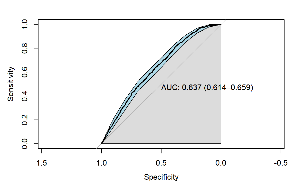

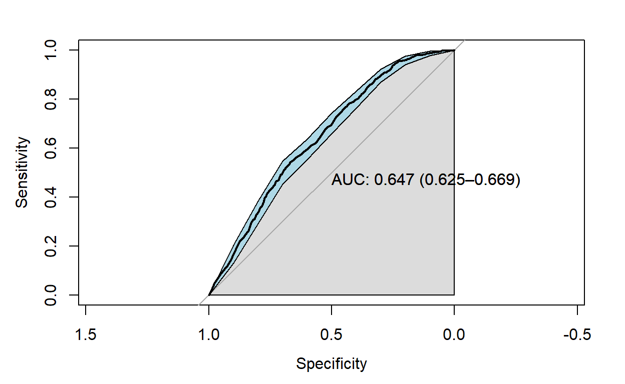
Now recall the logistic regression model that used age as a categorical variable. Is this model adequate according to the Hosmer-Lemeshow test

hltest(model4)


   The Hosmer-Lemeshow goodness-of-fit test

 Group Size Observed   Expected
     1  364        7   7.615801
     2  435       16  15.384199
     3  463       38  40.337537
     4  319       34  36.275270
     5  269       37  30.947529
     6  588       66  70.682056
     7  485       66  62.964352
     8  548       96  98.892386
     9  553      110 105.317944
    10  491      100 101.582924

         Statistic =  2.63554 
degrees of freedom =  8 
           p-value =  0.95511

What is the area under the ROC curve for this model?

Create an age² term and add this to the model with age as a continuous variable. Does adding this quadratic term improve the fit of the model?

Obviously it will improve the fit, but whether it is worth the added complexity is another question.

modelq <- update(model2, ~ . + I(age^2))
epicourse$age2 <- epicourse$age^2
summary(modelq)


Call:
glm(formula = hip_p == "yes" ~ sex + age + I(age^2), family = binomial("logit"), 
    data = epicourse)

Deviance Residuals: 
    Min       1Q   Median       3Q      Max  
-0.6809  -0.5912  -0.5124  -0.2951   3.1901  

Coefficients:
              Estimate Std. Error z value Pr(>|z|)    
(Intercept) -6.8154736  0.6747805 -10.100  < 2e-16 ***
sexM        -0.5499348  0.0932640  -5.897 3.71e-09 ***
age          0.1523200  0.0224885   6.773 1.26e-11 ***
I(age^2)    -0.0010601  0.0001827  -5.802 6.56e-09 ***
---
Signif. codes:  0 '***' 0.001 '**' 0.01 '*' 0.05 '.' 0.1 ' ' 1

(Dispersion parameter for binomial family taken to be 1)

    Null deviance: 3424.1  on 4514  degrees of freedom
Residual deviance: 3258.0  on 4511  degrees of freedom
AIC: 3266

Number of Fisher Scoring iterations: 6

hltest(modelq)


   The Hosmer-Lemeshow goodness-of-fit test

 Group Size Observed  Expected
     1  445        8  7.817101
     2  440       18 23.017377
     3  453       42 39.813627
     4  465       55 53.071191
     5  464       63 58.388841
     6  472       59 61.183630
     7  455       66 65.503783
     8  435       83 80.525915
     9  447       93 90.168478
    10  439       83 90.510057

         Statistic =  2.86936 
degrees of freedom =  8 
           p-value =  0.94229

Obtain the area under the ROC curve for this model. How does it compare for the previous models you considered?

Using the same procedure as above, we obtain the AUC:

Diagnostics

It is not easy to replicate Stata’s diagnostics in R

Produce a scatter plot of $\Delta\hat\beta_i$ against `fitted` values for the previous regression model. Is there any evidence of an influential point?

Pregibon’s $\Delta\hat\beta_i$ statistic, according to the Stata documentation, has the formula $\Delta\hat\beta_i = \frac{r_j^2 h_j}{(1 - h_j)^2},$ where $r_j$ is the Pearson residual for the $j^\text{th}$ observation and $h_j$ is the $j^\text{th}$ diagonal element of the hat matrix.

Unfortunately, calculating it is not straightforward, as R and stata differ about what a Pearson residual is and what the hat matrix is. And I could not find a package that did it. Don’t worry if you don’t understand what the function pregibon is doing below: I’m not sure I do (``I’’ here being ML, not DS :-)). However, it does duplicate the statistics produced by Stata.

pregibon <- function(model) {
  # This is very similar to Cook's distance
  Y <- tapply(model$y, list(model$model$sex, model$model$age), sum)
  M <- tapply(model$y, list(model$model$sex, model$model$age), length)
  vY <- diag(Y[as.character(model$model$sex), as.character(model$model$age)])
  vM <- diag(M[as.character(model$model$sex), as.character(model$model$age)])
  pr <- (vY - vM*model$fitted.values)/sqrt(vM*model$fitted.values*(1-model$fitted.values))
  V <- vcov(model)
  X <- cbind(rep(1, 4515), model$model$sex=="M", model$model$age, model$model$age*model$model$age)
  uhat <- diag(X %*% V %*% t(X))
  hat <- uhat*vM*model$fitted.values*(1-model$fitted.values)
  db <- (pr^2*hat)/(1-hat)^2
}
plot(fitted(modelq), pregibon(modelq), type = 'h')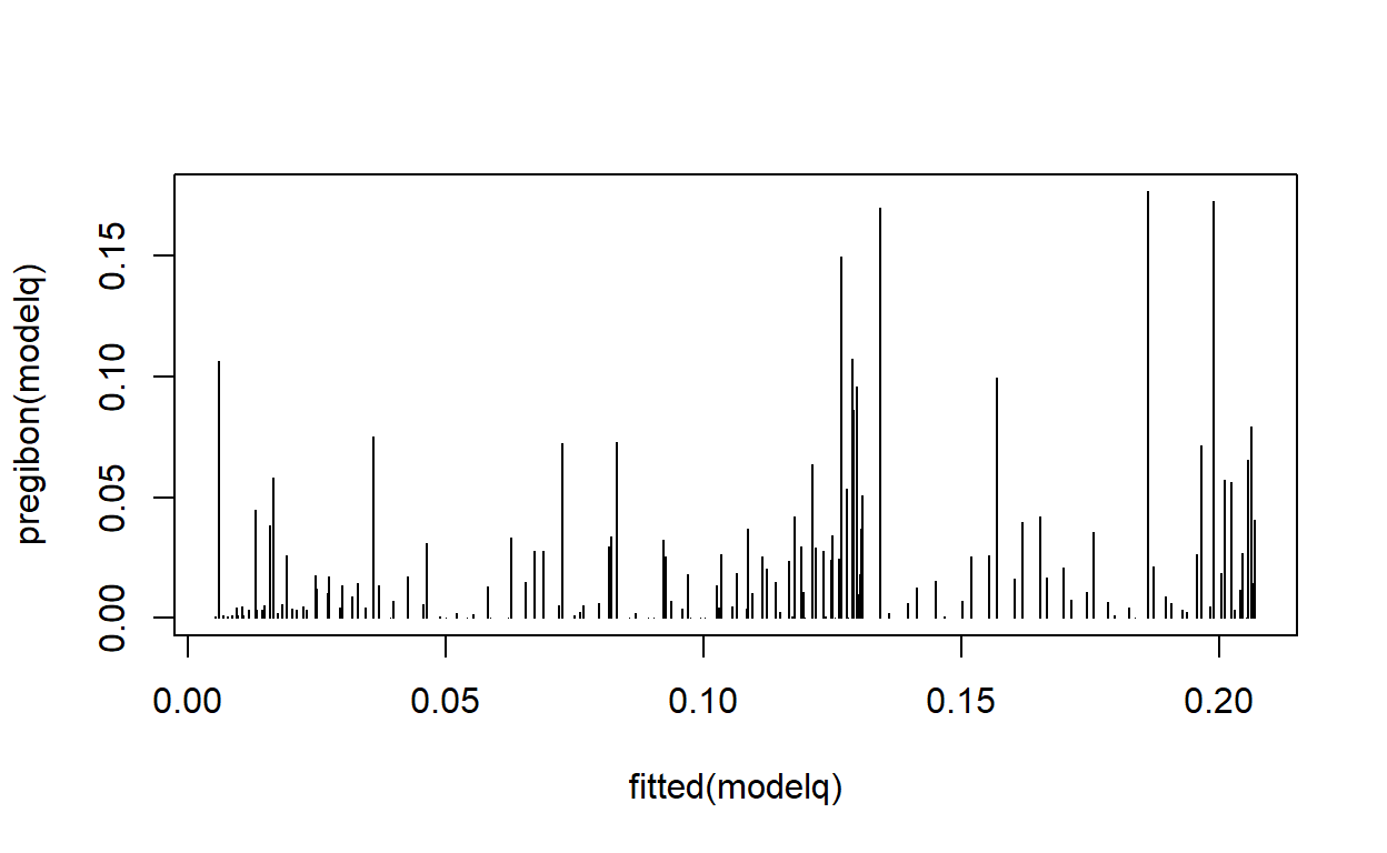

# You could compare this to Cook's distance using the command below, but Cook's distance does not have an
# interpretation for logistic regression, only linear regression
# plot(modelq, which = 4)

Obtain the deviance residuals and plot them against the fitted values. Is there evidence of a poor fit for any particular range of predicted values?

Deviance residuals are accessible via residuals(model, type = 'deviance').

plot(fitted(modelq), residuals(modelq, type = 'deviance'),
     xlab = 'Fitted values', ylab = 'Deviance residuals')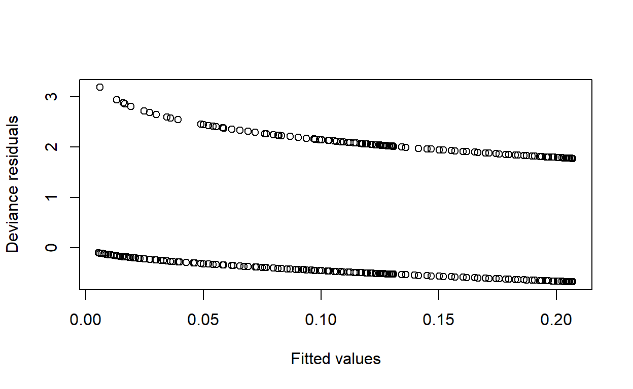

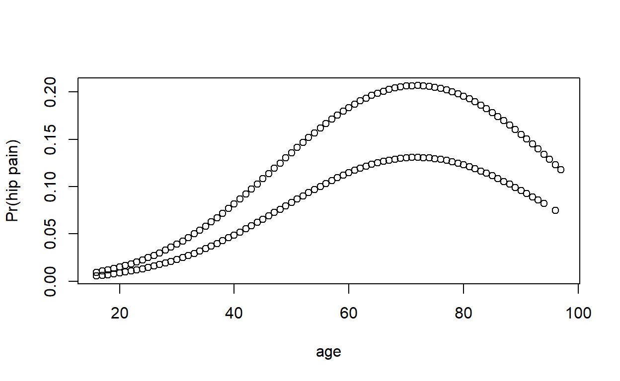
Plot fitted values against age. Why are there two curves?

plot(epicourse$age, fitted(modelq), xlab = 'age', ylab = 'Pr(hip pain)')

Compare logistic regression model predictions to a non-parametric smoothed curve.

You can use loess(), or geom_smooth() in ggplot2. If you are having trouble, try adjusting the smoothing parameter (span), and make sure the variables are in a numeric/binary format, as loess() doesn’t really like factors.

if(require(ggplot2)==FALSE) {
  install.packages(ggplot2)
  library(ggplot2)
}

ggplot(epicourse) +
  aes(age, as.numeric(hip_p) - 1) +
  geom_point(aes(y = fitted(modelq))) +
  geom_smooth(aes(colour = sex), method = 'loess', se = F, span = .75) +
  ylab('Pr(hip pain)')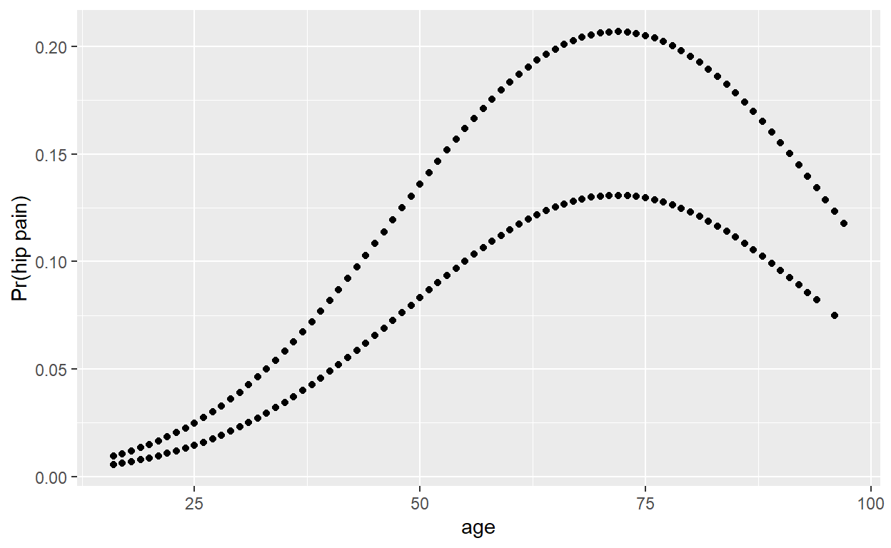

nonpar <- loess(data = transform(epicourse,
                                 pain = as.numeric(hip_p == 'yes'),
                                 male = as.numeric(sex == 'M')),
                pain ~ age * male, span = .75)
plot(epicourse$age, fitted(modelq), xlab = 'Age', ylab = 'Pr(hip pain)')
lines(1:100, predict(nonpar, newdata = data.frame(age = 1:100, male = T)), col = 'steelblue')
lines(1:100, predict(nonpar, newdata = data.frame(age = 1:100, male = F)), col = 'tomato2')
legend('topleft', lty = 1, col = c('steelblue', 'tomato2'), legend = c('M', 'F'))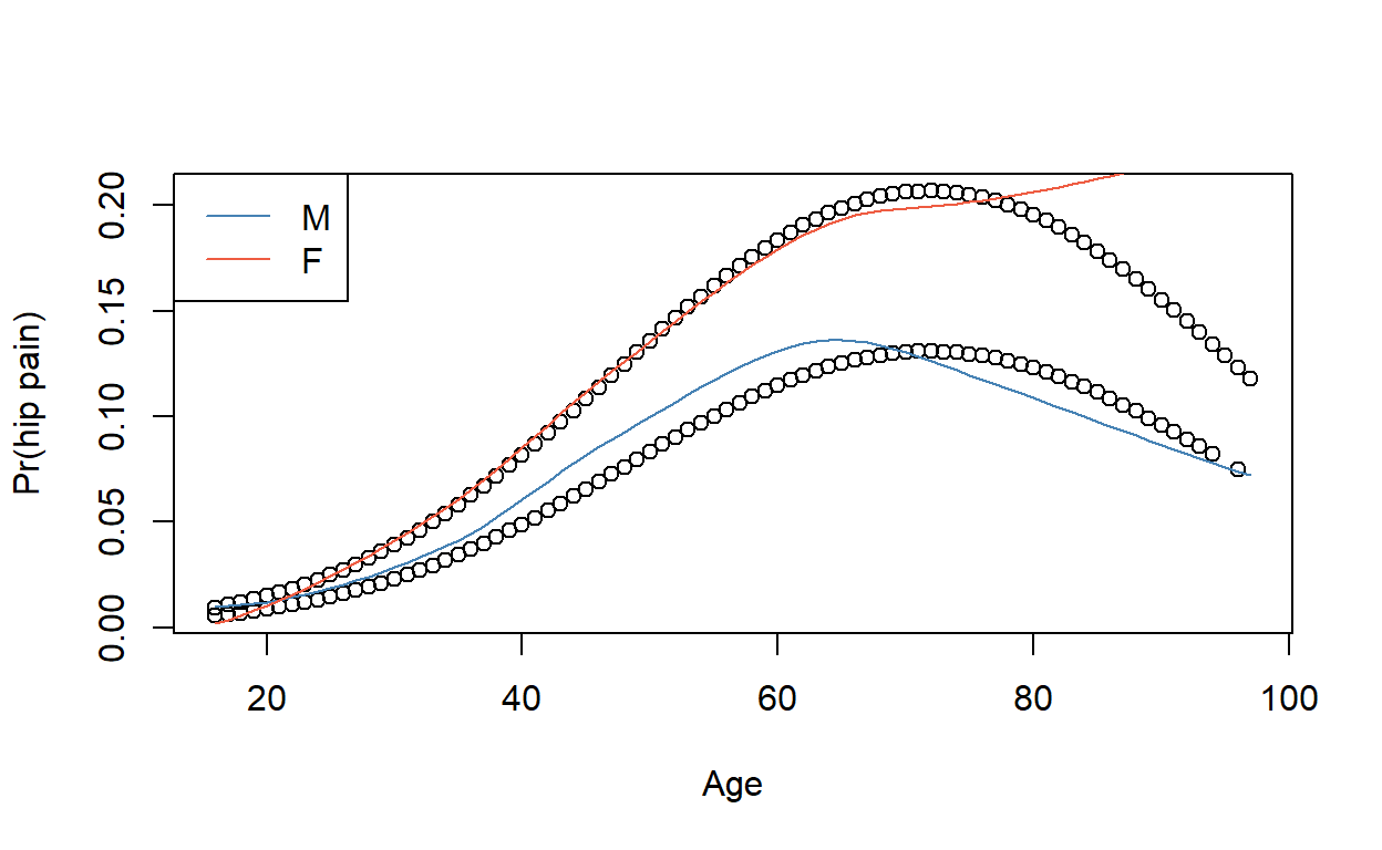

The CHD data

This section of the practical gives you the opportunity to work through the CHD example that was used in the notes.

chd <- read.csv('chd.csv')

The following commands will reproduce Figure 1.2 using base R:

chd_means <- aggregate(cbind(age, chd) ~ agegrp, mean, data = chd)
plot(chd ~ age, data = chd_means,
     xlab = 'Mean age', ylab = 'Proportion of subjects with CHD',
     main = 'Scatter plot of proportion of CHD against mean age')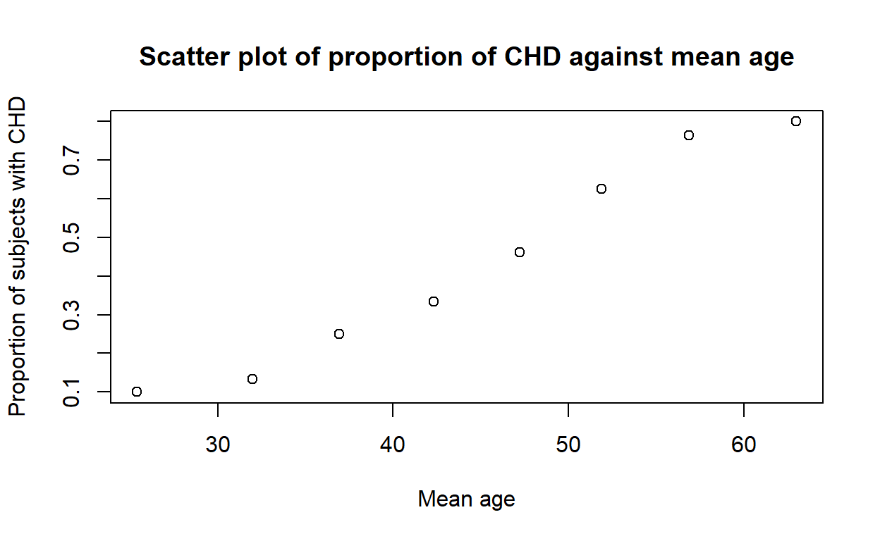

It can also be done in dplyr and ggplot2:

if (require(dplyr)==FALSE) {
  install.packages(dplyr)
  library(dplyr)
}
chd %>%
  group_by(agegrp) %>%
  summarise(agemean = mean(age),
            chdprop = mean(chd)) %>%
  ggplot() + aes(agemean, chdprop) +
  geom_point() +
  labs(x = 'Mean age', y = 'Proportion of subjects with CHD',
       main = 'Scatter plot of proportion of CHD against mean age')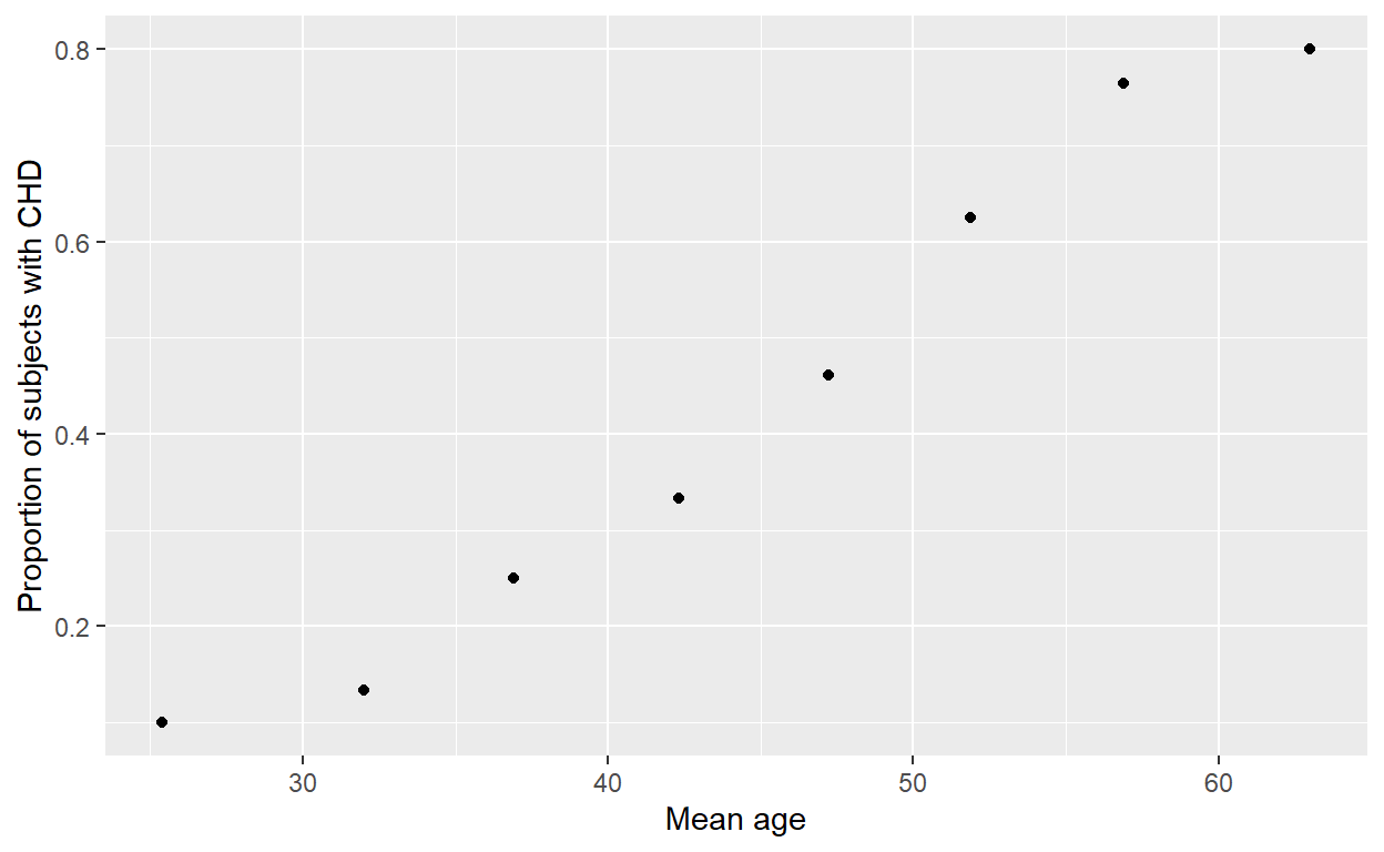

Fit the basic logistic regression model with `chd ~ age`. What is the odds ratio for a 1 year increase in age?

chd_model <- glm(chd ~ age, data = chd, family = binomial)
exp(coef(chd_model)['age'])

     age 
1.117307

Plot Pregibon’s $\Delta\hat\beta_i$ against the fitted values for this model. Are any points particularly influential?

chd_pregibon <- function(model) {
  Y <- tapply(model$y, list(model$model$age), sum)
  M <- tapply(model$y, list(model$model$age), length)
  vY <- Y[as.character(model$model$age)]
  vM <- M[as.character(model$model$age)]
  pr <- (vY - vM*model$fitted.values)/sqrt(vM*model$fitted.values*(1-model$fitted.values))
  V <- vcov(model)
  X <- cbind(rep(1, 100), model$model$age)
  uhat <- diag(X %*% V %*% t(X))
  hat <- uhat*vM*model$fitted.values*(1-model$fitted.values)
  db <- (pr^2*hat)/(1-hat)^2
}
db <- chd_pregibon(chd_model)
plot(fitted(chd_model), db, type = 'h')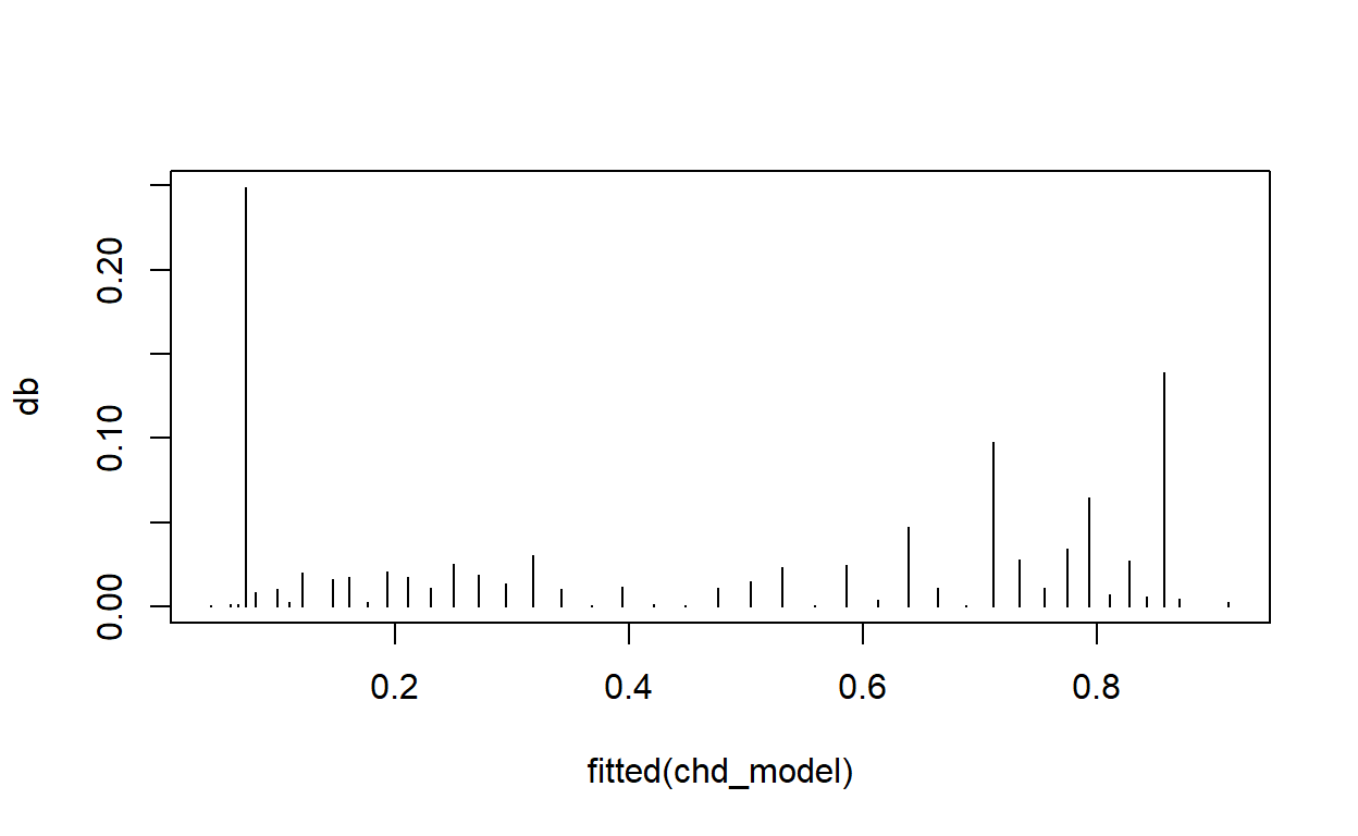

# plot(chd_model, which = 4)

chd_model <- glm(chd ~ age, data = chd[db < 0.2, ], family = binomial)
exp(coef(chd_model)['age'])

     age 
1.130329