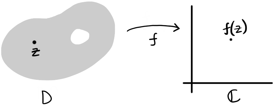
Figure 1: A function defined on a domain $D$ maps each complex number $z \in D$ to a complex number $f(z) \in \C$.
Home | Assessment | Notes | Index | Worksheets | Blackboard
Our main objects of study in this course are complex-valued functions $f$ where the inputs come from a domain $D \subset \mathbb{C}$. We will mainly be interested in differentiating and integrating such functions.
Figure 1: A function defined on a domain $D$ maps each complex number $z \in D$ to a complex number $f(z) \in \C$.
Often, functions are defined by formulae.
More complicated functions such as trigonometric and exponential functions will be formally defined by power series later on in the course. A complex version of the natural logarithm will have to wait until we have discussed integration!
Given a function $f : D \to \C$ we can think of $D$ as a subset of $\R^2$ and of $\C$ as the whole plane $\R^2$. Writing $z = x+iy$ and \[f(z) = f(x+iy) = u(x,y) + i v(x,y)\] lets us think of $f$ as being made up of two real-valued functions $u,v : D \to \R$.
What are the real and imaginary parts of $f(z) = z^2$? Writing $z = x+iy$ we have \[f(x+iy) = (x+iy)^2 = x^2 - y^2 + 2xyi\] so $u(x,y) = x^2 - y^2$ and $v(x,y) = 2xy$.
We cannot easily draw the graph of a function $f : D \to \C$. We conclude this section with a brief discussion of two alternative methods for visualizing such a function.
The first method is to plot the level curves of the real and imaginary parts $u$ and $v$ of $f : D \to \C$. Recall that the level curves of a function $h : D \to \R$ are the curves $h(x,y) = k$ for different values of $k$. We plot level curves in the domain of the function. If the input $z$ is nudged along a level curve of $u$ the real part of the output will not change. Similarly, if the input is nudged along a level curve of $v$ then the imaginary part of the output will not change.
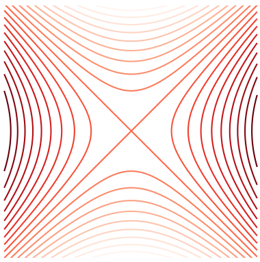
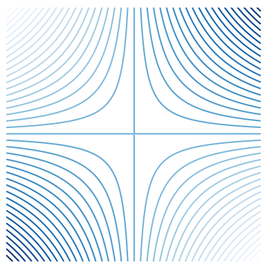
Figure 2: The level curves of the real and imaginary parts $u(x,y) = x^2 - y^2$ and $v(x,y) = 2xy$ of $f(z) = z^2$ respectively.
The second method is to think of $f$ as a vector field on $D$. Indeed, for every $z \in D$ the output $f(z)$ can be thought of as a vector in $\R^2$. Placing the tail of this vector at the point $z \in D$ lets us think of $f$ as a vector field on $D$.
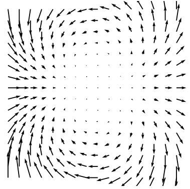
Figure 3: The function $f(z) = z^2$ as the vector field $\langle x^2-y^2, 2xy \rangle$ on $\R^2$.