This worksheet is based on the ninth lecture of the Statistical Modelling in Stata course, created by Dr Mark Lunt and offered by the Centre for Epidemiology Versus Arthritis at the University of Manchester. The original Stata exercises and solutions are here translated into their R equivalents.
Refer to the original slides and Stata worksheets here.
Though the original datasets were in the Stata-specific .dta mode, I have converted them for you into the more universal .csv format. Thus you can import them using the built-in read.csv or read.table functions (or the method of your choice).
Poisson regression
In this section you will be analysing the dataset ships provided in the MASS (Modern Applied Statistics with S) package. This is data from Lloyds of London concerning the rate at which damage occurred at different times to different types of ship.
There are five types of ship (labelled “A” to “E”), which could have been built in any one of four time periods (year), and sailed during one of two time periods. The aggregate duration of operation of each type of ship (in months) is given by service, and the number of incidents of damage is given by incidents.
data(ships, package = 'MASS')
Familiarise yourself with the meanings of the variables.
help(ships, package = 'MASS')
Convert the columns period, type and year to factor (if they are not already) and set the reference level of type to “E” and year to “75” (1975–1979) with the relevel function.
Are there any differences in the rates at which damage occurs according to the type of ship?
Fit a generalised linear model with a logarithmic link function. The R equivalent of Stata’s exposure in a log-linear model is to wrap the log of the variable in offset() on the right-hand side of the model formula.
Obviously we can’t take logarithms of zero, so ignore classes of ships that did not see any service (using subset in glm, or otherwise by removing these rows from the data frame).
So we don’t have to write this out repeatedly, we’ll create a model just for the offset term and then generate our other models by adding terms with update().
model_null <- glm(incidents ~ offset(log(service)), family = poisson,
                  data = ships, subset = service > 0)
model_type <- update(model_null, ~ . + type)
anova(model_type)
Analysis of Deviance Table

Model: poisson, link: log

Response: incidents

Terms added sequentially (first to last)

     Df Deviance Resid. Df Resid. Dev
NULL                    33    146.328
type  4   55.439        29     90.889
Unlike lm objects, when you apply anova to glm objects in R it doesn’t automatically perform the test for you. But you can carry it out yourself.
The \(\chi^2\) test statistic is 55.4 on 4 degrees of freedom, giving a p-value of
pchisq(deviance(model_null) - deviance(model_type),       # = 55.4
       df.residual(model_null) - df.residual(model_type), # = 4
       lower.tail = FALSE)
[1] 2.628688e-11which is effectively zero, hence the type term is highly significant.
Note. In this case, anova(model_type) gives equivalent output to anova(model_null, model_type).
Are there any differences in the rates at which damage occurs according to the time at which the ship was built?
model_built <- update(model_null, ~ . + year)
anova(model_built) # or anova(model_null, model_built)
Analysis of Deviance Table

Model: poisson, link: log

Response: incidents

Terms added sequentially (first to last)

     Df Deviance Resid. Df Resid. Dev
NULL                    33    146.328
year  3   73.103        30     73.225
The year term is highly significant and once again gives a p-value of near-zero. (You can verify this using the method given in the previous question.)
Are there any differences in the rates at which damage occurs according to the time in which the ship was operated?
Analysis of Deviance Table

Model: poisson, link: log

Response: incidents

Terms added sequentially (first to last)

       Df Deviance Resid. Df Resid. Dev
NULL                      33     146.33
period  1   33.563        32     112.77
Again the term is highly significant.
Now add all three variables into a multivariate Poisson model. Test if ship type is significant after adjusting for the other predictors.
Applying the function anova(model) implicitly compared model with the null. Here we want to compare the full model with one that includes every term except type. We use the anova(model1, model2) syntax to get the corresponding \(\chi^2\) test statistic.
model_full <- glm(incidents ~ offset(log(service)) + year + period + type,
                  family = poisson,
                  data = ships, subset = service > 0)
model_built_sailed <- update(model_full, ~ . - type)
anova(model_built_sailed, model_full)
Analysis of Deviance Table

Model 1: incidents ~ year + period + offset(log(service))
Model 2: incidents ~ offset(log(service)) + year + period + type
  Resid. Df Resid. Dev Df Deviance
1        29     62.365
2        25     38.695  4    23.67
The resulting p-value is therefore
pchisq(deviance(model_built_sailed) - deviance(model_full),
       df.residual(model_built_sailed) - df.residual(model_full),
       lower.tail = FALSE)
[1] 9.299568e-05which implies that the effect of ship type is still significant after the other factors are taken into account.
Use function fitted (or predict) to obtain expected numbers of damage incidents. Compare the observed and expected numbers of incidents. For which type of ship and which time periods are the predicted values furthest from the observed values?
The canonical Stata-like solution translated to R is something like
And then inspecting the resulting data frame (the last rows thereof) either using View or tail to see which type and time periods had the largest magnitude residuals.
In dplyr the equivalent operations are:
You can also get the residuals directly (rather than doing the subtraction yourself) using the residuals (aka resid) accessor function on the model object.
residuals(model_full, type = 'response')
So you can retrieve the desired row using
ships <- subset(ships, service > 0)
ships <- transform(ships,
                   pred_n = fitted(model_full),
                   resid = residuals(model_full, 'response'))
ships[which.max(abs(ships$resid)), ]
   type year period service incidents   pred_n    resid
30    D   70     75    1208        11 6.157999 4.842001
And see that the least accurate prediction was for type D ships built in 1970–1974, operated in 1975–1979, with 11 damage incidents observed and 6.2 predicted by the model.
Test whether the model is adequate.
The Stata command estat gof provides goodness-of-fit statistics for the model, which tests whether the observed and expected values are significantly different from one another.
The residual deviance is mentioned in the last line of output from summary(model_full). The resulting p-value from the \(\chi_{25}^2\) test is
pchisq(deviance(model_full), # sum(resid(model_full, 'deviance')^2)
       df.residual(model_full),
       lower.tail = FALSE)
[1] 0.03951433Pearson’s cumulative test statistic (the other output of Stata’s estat gof) is
which has 25 degrees of freedom, giving a p-value of 0.017.
We therefore reject the null hypothesis that the observed data are drawn from the distribution specified by the fitted model. In other words, the model is not a great fit.
Add a term of the interaction between ship type and year of operation. Test whether this term is statistically significant.
Note. The original Stata solution sheet appears to be wrong here, as it interacts ship type with built, rather than sailed, as asked in the question. First we will add the type:built interaction term, then later on we will answer the original question.
Analysis of Deviance Table

Model 1: incidents ~ offset(log(service)) + year + period + type
Model 2: incidents ~ year + period + type + year:type + offset(log(service))
  Resid. Df Resid. Dev Df Deviance
1        25     38.695
2 13 14.587 12 24.108pchisq(deviance(model_full) - deviance(inter_built),
df.residual(model_full) - df.residual(inter_built),
lower.tail = FALSE)
[1] 0.01966268The interaction between year built and type of ship is significant. The goodness-of-fit statistic yields \(\chi_{13}^2\) = 14.6, with p-value
pchisq(deviance(inter_built),
       df.residual(inter_built),
       lower.tail = FALSE)
[1] 0.3338479implying that the model is now a good fit.
Testing for the year of operation (as was originally asked in the question):
Analysis of Deviance Table

Model 1: incidents ~ offset(log(service)) + year + period + type
Model 2: incidents ~ year + period + type + period:type + offset(log(service))
  Resid. Df Resid. Dev Df Deviance
1        25     38.695
2        21     33.756  4   4.9388
The interaction term between year of operation and type of ship is not significant, so it does not appear to be worth adding that to the model.
pchisq(deviance(model_full) - deviance(inter_sailed),
       df.residual(model_full) - df.residual(inter_sailed),
       lower.tail = FALSE)
[1] 0.2936317Negative binomial regression
This section uses data concerning childhood mortality in three cohorts, from the dataset nbreg.csv. The children were divided into seven age bands1, and the number of deaths, and the persons-months of exposure are recorded in deaths and exposure respectively.
nbreg <- read.csv('nbreg.csv')
Fit a Poisson regression model using only cohort as a predictor. Are there differences in mortality rate between the cohorts?
Firstly, convert cohort to a factor, so it doesn’t get misinterpreted as a continuous variable.
nbreg$cohort <- as.factor(nbreg$cohort)
Then, fit the generalised linear model.
pois_mod <- glm(deaths ~ offset(log(exposure)) + cohort,
                data = nbreg, family = poisson)
summary(pois_mod)
Call:
glm(formula = deaths ~ offset(log(exposure)) + cohort, family = poisson,
    data = nbreg)

Deviance Residuals:
    Min       1Q   Median       3Q      Max
-18.697   -7.419    4.800    8.253   31.485

Coefficients:
            Estimate Std. Error z value Pr(>|z|)
(Intercept) -3.89949    0.04113 -94.799  < 2e-16 ***
cohort2     -0.30204    0.05733  -5.268 1.38e-07 ***
cohort3      0.07421    0.05897   1.258    0.208
---
Signif. codes:  0 '***' 0.001 '**' 0.01 '*' 0.05 '.' 0.1 ' ' 1

(Dispersion parameter for poisson family taken to be 1)

    Null deviance: 4239.8  on 20  degrees of freedom
Residual deviance: 4190.7  on 18  degrees of freedom
AIC: 4325

Number of Fisher Scoring iterations: 6
There’s no point actually trying to interpret the coefficients, for reasons explained in the next question.
Was a Poisson model appropriate? If not, why not?
We want to check for overdispersion in the model. A Poisson model is overdispersed (or underdispersed) if the variance is significantly greater (or smaller) than the mean. This is indicated by the ratio of deviance to residual degrees of freedom being different from 1.
You can calculate the overdispersion parameter, which has definition \[\hat\phi = \sum_{i=1}^n \frac{r^2} {n - p + 1},\] the sum of the squared Pearson residuals divided by the residual degrees of freedom. Here we have
sum(residuals(pois_mod, 'pearson')^2) / df.residual(pois_mod)
[1] 854.8705which you can also verify by fitting the same model with family = quasipoisson and looking at the dispersion parameter given in the model summary output.
Clearly, our model is very overdispersed, meaning the variance is much larger than the mean, and so the Poisson model is not appropriate.
Fit a negative binomial regression model to test the same hypothesis.
We can use the function glm.nb from the MASS package.
library(MASS)
nb_model <- glm.nb(deaths ~ offset(log(exposure)) + cohort, data = nbreg)
summary(nb_model)
Call:
glm.nb(formula = deaths ~ offset(log(exposure)) + cohort, data = nbreg,
    init.theta = 0.5521163589, link = log)

Deviance Residuals:
    Min       1Q   Median       3Q      Max
-1.7820  -1.2812  -0.5685  -0.3042   1.6560

Coefficients:
            Estimate Std. Error z value Pr(>|z|)
(Intercept)  -2.0867     0.5099  -4.092 4.27e-05 ***
cohort2      -0.2676     0.7211  -0.371    0.711
cohort3      -0.4574     0.7211  -0.634    0.526
---
Signif. codes:  0 '***' 0.001 '**' 0.01 '*' 0.05 '.' 0.1 ' ' 1

(Dispersion parameter for Negative Binomial(0.5521) family taken to be 1)

    Null deviance: 26.618  on 20  degrees of freedom
Residual deviance: 26.212  on 18  degrees of freedom
AIC: 270.76

Number of Fisher Scoring iterations: 1

              Theta:  0.552
          Std. Err.:  0.143

 2 x log-likelihood:  -262.760
There are no significant differences between cohorts. (Similarly, anova(nb_model) shows variation between cohorts is not significantly greater than within cohorts.)
What is the value of the parameter \(\alpha\) and its 95% confidence interval?
This refers to the model formulation \[\text{Var}(Y) = \mu(1 + \alpha \mu)\] mentioned in the lecture notes, hence \(\alpha\) is the dispersion parameter for the quasi-negative binomial model.
Be aware that the MASS::glm.nb summary output defines the dispersion parameter differently, with \[\text{Var}(Y) = \mu + \frac{\mu^2}{\theta}.\] A full explanation is given here. The dispersion parameter \(\alpha\) is therefore:
1 / nb_model$theta
[1] 1.811212or you can compute it yourself:
A confidence interval for \(\theta = 1/\alpha\) is
nb_model$theta + c(-1, 1) * 1.96 * nb_model$SE.theta
[1] 0.2725365 0.8316963Fit a constant dispersion negative binomial regression model. Is \(\delta\) significantly greater than 0 in this model ?
From the lecture notes, this refers to the model parametrisation \[\text{Var}(Y) = \mu(1 + \delta),\] which is similar to the quasi-Poisson \[\text{Var}(Y) = \phi\mu,\] for a dispersion parameter \(\phi\).
According to Brian Ripley, the Stata command nbreg with option dispersion(constant) is not fitting a GLM at all. The constant-dispersion negative binomial described in Stata is possibly(?) analogous to a quasi-Poisson. However the dispersion parameter given in summary(qpois_model) is much larger than that given in the Stata solutions, so I’m not 100% sure. More details are in the Stata documentation.
One possible source of the extra variation is a change in mortality with age. Fit a model to test whether mortality varies with age.
(Since cohort was not sigificant, it is dropped for this model.)
nb_null <- glm.nb(deaths ~ offset(log(exposure)), data = nbreg)
nb_age <- update(nb_null, ~ . + age_gp)
anova(nb_null, nb_age)
Likelihood ratio tests of Negative Binomial Models

Response: deaths
                           Model      theta Resid. df    2 x log-lik.
1          offset(log(exposure))  0.5448456        20       -263.1637
2 age_gp + offset(log(exposure)) 32.8191113        14       -174.6108
    Test    df LR stat.      Pr(Chi)
1
2 1 vs 2     6 88.55287 1.110223e-16
The likelihood ratio test statistic is 2 × 44 on 6 degrees of freedom, which is highly significant, suggesting mortality is different between age groups.
Would it be appropriate to use a Poisson regression to fit this model?
No, because \(\theta = \alpha^{-1} = 33 ~ (= 0.03^{-1})\), indicating overdispersion.
Now fit a negative binomial regression model with both age and cohort as predictors. Determine whether both age and cohort are independently significant predictors of mortality.
As in Stata, this model struggles to converge. You can try to tweak the model fitting hyperparameters in glm.control.
nb_age_cohort <- update(nb_age, ~ . + cohort) # throws lots of warnings
Or better yet, fit the model using Markov chain Monte Carlo (MCMC) via Stan.
library(rstanarm)
nb_age_cohort <- stan_glm.nb(deaths ~ age_gp + cohort, offset = log(exposure),
                             data = nbreg, algorithm = 'sampling')
The 90% Bayesian posterior uncertainty (“credible”) intervals are:
posterior_interval(nb_age_cohort)
                              5%         95%
(Intercept)           -0.8894062  0.05812199
age_gp1 - 2 years     -3.5563989 -2.37902713
age_gp1 - 3 months    -2.5086262 -1.33259101
age_gp2 - 5 years     -4.6454879 -3.47878564
age_gp3 - 6 months    -2.7096605 -1.49816111
age_gp5 - 10 years    -5.9977367 -4.78428108
age_gp6 - 12 months   -3.0297717 -1.86654274
cohort2               -0.7329776  0.03835061
cohort3               -0.8779173 -0.07631221
reciprocal_dispersion  3.1187818 10.87741584
which do not contain zero for the age or cohort parameters, implying that age and cohort have an effect on mortality.
Is there overdispersion in this model?
The 95% credible interval for the reciprocal dispersion is
posterior_interval(nb_age_cohort, par = 'reciprocal_dispersion', prob = .95)
                         2.5%    97.5%
reciprocal_dispersion 2.72359 11.80151
which are both greater than one, implying there is, if anything, underdispersion in the model, but no longer overdispersion.
Fit the same model using family = poisson. Does this model agree with the negative binomial model?
“Fit the same model using (different model spec)” is maybe an odd way of phrasing this! Anyway, the equivalent Poisson model (back to using stats::glm again) is
Call:
glm(formula = deaths ~ cohort + age_gp + offset(log(exposure)),
    family = poisson, data = nbreg)

Deviance Residuals:
     Min        1Q    Median        3Q       Max
-1.08117  -0.35186  -0.00218   0.35059   0.81597

Coefficients:
                    Estimate Std. Error z value Pr(>|z|)
(Intercept)         -0.44847    0.05454  -8.223  < 2e-16 ***
cohort2             -0.32426    0.05734  -5.655 1.55e-08 ***
cohort3             -0.47841    0.05933  -8.064 7.37e-16 ***
age_gp1 - 2 years   -3.01404    0.07270 -41.457  < 2e-16 ***
age_gp1 - 3 months  -1.97267    0.09170 -21.513  < 2e-16 ***
age_gp2 - 5 years   -4.11538    0.07583 -54.274  < 2e-16 ***
age_gp3 - 6 months  -2.16334    0.08515 -25.407  < 2e-16 ***
age_gp5 - 10 years  -5.43589    0.11477 -47.364  < 2e-16 ***
age_gp6 - 12 months -2.49168    0.07555 -32.980  < 2e-16 ***
---
Signif. codes:  0 '***' 0.001 '**' 0.01 '*' 0.05 '.' 0.1 ' ' 1

(Dispersion parameter for poisson family taken to be 1)

    Null deviance: 4239.849  on 20  degrees of freedom
Residual deviance:    6.182  on 12  degrees of freedom
AIC: 152.53

Number of Fisher Scoring iterations: 3
This appears to agree with the negative binomial model: all terms are significant and the parameter estimates are almost identical to those given in the model nb_age_cohort. Moreover, the residual deviance implies no overdispersion (though possibly underdispersion).
Perform a goodness-of-fit test.
pchisq(deviance(pois_age_cohort), df.residual(pois_age_cohort),
       lower.tail = FALSE)
[1] 0.9066301No longer significant, implying a good fit.
Using constraints
This section uses the data on damage to ships from the dataset MASS::ships, again.
Refit (or retrieve) the final Poisson regression model considered in the first section. Which of the incidents rate ratios are not significantly different from 1?
In R, the standard output returns log-incidence ratios, so you can either apply exp to the coefficients to get relative incidence ratios, or else on the logarithmic scale check which parameters’ confidence intervals contain zero (\(\log 1 = 0\)).
If you’re working in the same R session as before, you should still have type “E” and construction year 1975–1979 as reference levels, resulting in output like below. (If your reference levels are construction year 1960–1964 and type “A”, you can still make the same inferences, but the output will look different.)
ship_model <- glm(incidents ~ offset(log(service)) + year + period + type,
                  family = poisson(link = 'log'),
                  data = ships, subset = service > 0)
confint(ship_model)
             2.5 % 97.5 %
(Intercept) -6.178 -5.108
year60      -0.904  0.012
year65      -0.155  0.665
year70      -0.015  0.769
period75     0.153  0.617
typeA       -0.785  0.143
typeB       -1.244 -0.463
typeC       -1.718 -0.375
typeD       -1.025  0.187
Construction year 1960–1964 is not significantly different from 1975–1979 (though it’s borderline). Types A and D are not significantly different from type E.
Add a column of predicted numbers of damage incidents to your data frame.
ships$pred_n <- fitted(ship_model)
Define a constraint to force the incidence rate rate for ships of type D to be equal to 1.
In R, you accomplish this using contrasts. The default contrasts are contr.treatment, which means all comparisons are with the baseline factor level (type “A” by default, though we switched it to “E” in the first section).
contrasts(ships$type)
  A B C D
E 0 0 0 0
A 1 0 0 0
B 0 1 0 0
C 0 0 1 0
D 0 0 0 1ship_model$contrasts
$year
[1] "contr.treatment"

$period
[1] "contr.treatment"

$type
[1] "contr.treatment"
Assuming the question is not just asking us to change the reference level again (in which case we’d employ relevel()), we can construct a contrasts matrix where the reference level and type D have rows equal to zero.
How does the output of this model differ from the previous one?
summary(ship_model_D)
Call:
glm(formula = incidents ~ offset(log(service)) + year + period +
    type, family = poisson(link = "log"), data = ships, subset = service >
    0, contrasts = list(type = type_contr))

Deviance Residuals:
   Min      1Q  Median      3Q     Max
-1.839  -0.744  -0.389   0.370   2.777

Coefficients: (1 not defined because of singularities)
            Estimate Std. Error z value Pr(>|z|)
(Intercept)   -5.822      0.234  -24.84  < 2e-16 ***
year60        -0.412      0.232   -1.77   0.0760 .
year65         0.291      0.207    1.41   0.1587
year70         0.419      0.196    2.14   0.0320 *
period75       0.380      0.118    3.21   0.0013 **
typeA         -0.169      0.210   -0.80   0.4221
typeB         -0.716      0.170   -4.22  2.4e-05 ***
typeC         -0.863      0.324   -2.66   0.0078 **
typeD             NA         NA      NA       NA
---
Signif. codes:  0 '***' 0.001 '**' 0.01 '*' 0.05 '.' 0.1 ' ' 1

(Dispersion parameter for poisson family taken to be 1)

    Null deviance: 146.328  on 33  degrees of freedom
Residual deviance:  40.461  on 26  degrees of freedom
AIC: 154.3

Number of Fisher Scoring iterations: 5
The typeD row is now effectively blanked out, because the estimate is constrained to logit zero (relative incidence of 1) and has no standard error. The other parameter estimates have changed slightly, though not by a large amount. (Recall from earlier that the effect of type “D” is not statistically significant.)
Test the adequacy of this (constrained) model compared to the unconstrained model.
Both give very similar results and indicate a lack of fit:
# Original model:
pchisq(deviance(ship_model), df.residual(ship_model), lower = F)
[1] 0.04# With type D constraint:
pchisq(deviance(ship_model_D), df.residual(ship_model_D), lower = F)
[1] 0.035Define a second constraint to force the incidence ratio for ships of type E to be equal to 1.
If type “E” is still your reference category, it does not make much sense to force it to be zero, as it is already. Hence we will relevel the factor so that type “A” is the new reference category, then add the constraint.
# Reset factor levels to be alphabetical order
levels(ships$type) <- sort(levels(ships$type)) # or `LETTERS[1:5]`

# Make new contrasts matrix
type_contr <- contrasts(ships$type)
type_contr[c('D', 'E'), ] <- 0
type_contr
  B C D E
A 0 0 0 0
B 1 0 0 0
C 0 1 0 0
D 0 0 0 0
E 0 0 0 0
Fit a Poisson regression model with both of these constraints.
How does the adequacy of this model compare to that of the previous one?
pchisq(deviance(ship_model_DE),
       df.residual(ship_model_DE),
       lower.tail = F)
[1] 0.0064Lack of fit has got worse—this p-value is smaller than before.
It appears that the incidence rate ratio for being built in 1965–1969 is very similar to the incidence rate ratio for being built in 1970–1974. Define a new constraint to force these parameters to be equal.
As building contrasts matrices becomes more complex, you might like to look up packages to simplify the process. Here I’ll do it in base R. (I hope this is right!)
levels(ships$year) <- sort(levels(ships$year))
year_contr <- contrasts(ships$year)
year_contr[, c('65', '70')] <- c(0, 1, 1, 0) / 2
year_contr
    65  70 75
60 0.0 0.0  0
65 0.5 0.5  0
70 0.5 0.5  0
75 0.0 0.0  1
Fit a Poisson regression model with all three constraints:
In Stata’s model summary output, the lines for the constrained construction years would be identical. In R, summary(ship_model_constr) will instead show year70 as NA, since it is redundant. (Or, if we omit columns of zeros from the contrasts matrix, those rows will simply not appear.) Here, year65 still has a valid estimate and standard error, since it was not constrained to take a specific value (only to be equal to that of year70).
exp(cbind(estimate = coefficients(ship_model_constr),
          confint(ship_model_constr)))
            estimate  2.5 % 97.5 %
(Intercept)   0.0023 0.0015 0.0036
year65        0.9562 0.4426 2.1691
year70            NA     NA     NA
year75        1.4659 1.0125 2.1763
period75      1.5668 1.2434 1.9775
typeB         1.1050 0.7411 1.6320
typeC         0.6033 0.4490 0.8214
typeD             NA     NA     NA
typeE             NA     NA     NA
You can verify that they are treated the same (and that types “D” and “E” have no effect) by predicting on new data, for example:
predict(ship_model_constr,
        newdata = list(service = c(1, 1),
                       type = c('D', 'E'),
                       year = c('65', '70'),
                       period = c('75', '75')))
   1    2
-5.6 -5.6
What do you think is the reason for the difference you have just observed?
They were not constrained to take a specific value.
Test the adequacy of this constrained model. Have the constraints that you have applied to the model had a serious detrimental effect on the fit of the model?
pchisq(deviance(ship_model_constr),
       df.residual(ship_model_constr),
       lower.tail = F)
[1] 7.1e-06The fit has deteriorated slightly.
Obtain predicted counts from this constrained model.
ships$pred_cn <- fitted(ship_model_constr)
Compare the observed values with the predictions from the constrained and unconstrained models.
We can use a scatterplot matrix.
Tip. See help(pairs) for tips on how to get correlations in the same figure.
          incidents pred_n pred_cn
incidents      1.00   0.99    0.92
pred_n         0.99   1.00    0.94
pred_cn        0.92   0.94    1.00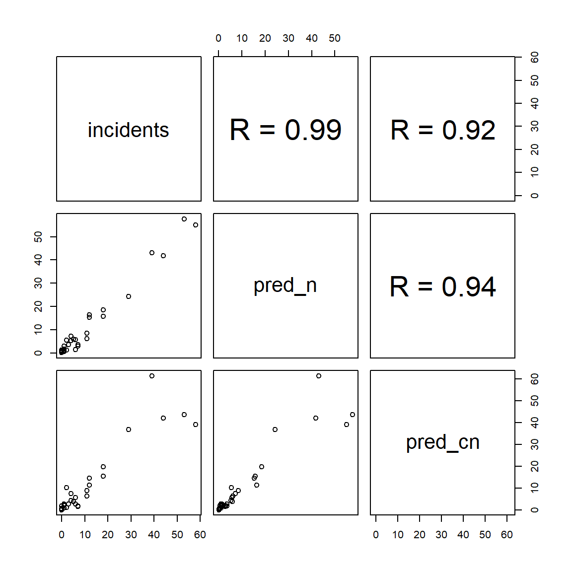
From this, it appears the constraints have had little effect on the fit of the model; the correlation between predicted and observed values is still very high (though it has dropped slightly).
If you wish, you can examine the observed and predicted values directly with View(ships) (or otherwise by printing them to the console).
Constraints in multinomial logistic regression
Constraints can be applied to many different types of regression model. However, applying constraints when using nnet::multinom can be tricky because there are several equations. The syntax is then similar to the syntax we saw last week for lincom.
For this part of the practical, we are using the same alligators.dta dataset that we saw last week.
Use levels or str to remind yourself of the different variables.
lapply(alligators, levels)
$lake
[1] "Hancock"  "Oklawaha" "Trafford" "George"

$gender
[1] "Male"   "Female"

$size
[1] "<= 2.3m" "> 2.3m"

$food
[1] "Fish"         "Invertebrate" "Reptile"      "Bird"
[5] "Other"
Fit a multinomial logistic regression model to predict food choice from lake with the function nnet::multinom().
mn_model <- nnet::multinom(food ~ lake, data = alligators)
Are there significant differences between lakes in the primary food choice?
# weights:  10 (4 variable)
initial  value 352.466903
final  value 302.181462
converged
Likelihood ratio tests of Multinomial Models
Response: food
Model Resid. df Resid. Dev Test Df LR stat. Pr(Chi)
1 1 872 604
2 lake 860 561 1 vs 2 12 43 2.1e-05Yes.
What are the odds ratios for preferring invertebrates to fish in Lakes Oklawaha, Trafford and George?
Fish is the reference food choice. So the odds ratios are
exp(coefficients(mn_model))['Invertebrate', ]
 (Intercept) lakeOklawaha lakeTrafford   lakeGeorge
        0.13         7.92        10.38         4.55
It appears that for the choice of invertebrates rather than fish, there is no significant difference between Lake Oklawaha and Lake Trafford. Define a corresponding constraint using contrasts.
lake_contrasts <- contrasts(alligators$lake)
lake_contrasts[, c('Oklawaha', 'Trafford')] <- c(0, 1, 1, 0) / 2
lake_contrasts
         Oklawaha Trafford George
Hancock       0.0      0.0      0
Oklawaha      0.5      0.5      0
Trafford      0.5      0.5      0
George        0.0      0.0      1
Fit the constrained model.
Look at the new parameter estimates:
exp(coefficients(mn_model2))
             (Intercept) lakeOklawaha lakeTrafford lakeGeorge
Invertebrate        0.13         8.95         8.95       4.55
Reptile             0.10         4.84         4.84       0.30
Bird                0.17         0.97         0.97       0.55
Other               0.43         0.97         0.97       0.42
(Unlike glm objects, redundant parameters in a multinom are repeated, rather than marked as NA.)
Even Lake George does not appear to be significantly different from Lake Oklawaha and Lake Trafford. Define another corresponding constraint.
lake_contrasts[] <- c(0, 1, 1, 1) / 3
lake_contrasts
         Oklawaha Trafford George
Hancock      0.00     0.00   0.00
Oklawaha     0.33     0.33   0.33
Trafford     0.33     0.33   0.33
George       0.33     0.33   0.33
Fit a multinomial logistic regression model with both of these constraints.
How does the common odds ratio for all three lakes compare to the 3 separate odds ratios you calculated previously?
exp(coefficients(mn_model3))
             (Intercept) lakeOklawaha lakeTrafford lakeGeorge
Invertebrate        0.13         6.68         6.68       6.68
Reptile             0.10         2.50         2.50       2.50
Bird                0.17         0.75         0.75       0.75
Other               0.43         0.69         0.69       0.69
The common odds ratio of 6.68 is somewhere in between the three previous estimates. Verify it with a single logistic regression:
logistic <- glm(food == 'Invertebrate' ~ lake != 'Hancock',
                data = alligators,
                subset = food %in% c('Invertebrate', 'Fish'),
                family = binomial)
exp(coefficients(logistic))
          (Intercept) lake != "Hancock"TRUE
                 0.13                  6.68
The original Stata 13
nbreg.dtafile containedage_gpas a column of labelled floating-point numbers. For cross-compatibility, I’ve converted this to a character vector.↩︎