This worksheet is based on the eighth lecture of the Statistical Modelling in Stata course, created by Dr Mark Lunt and offered by the Centre for Epidemiology Versus Arthritis at the University of Manchester. The original Stata exercises and solutions are here translated into their R equivalents.
Refer to the original slides and Stata worksheets here.
The datasets for this practical can be accessed via http from within R. The file path is very long, so you can save yourself some typing by saving it to a variable. The function file.path joins strings together with slashes, for example if you want to combine a web address with a directory or file name.
As Mark has saved these datasets in the Stata-specific .dta format, we import them into R using the read.dta function from the foreign package. Usually however, data are stored in CSV format and they can be imported with the base function read.csv.
Binomial and multinomial logistic regression
The data used for this section was collected as part of a survey of alligator food choices in 4 lakes in Florida. The largest contributor to the volume of the stomach contents was used as the outcome variable food, and the characteristics of the alligators are their length (dichotomised as ≤ 2.3m and > 2.3m), their sex and which of the four lakes they were caught in.
Load the alligators.dta data into R from the path above.
Familiarise yourself with the factor labels in the dataset. For example, since every column is a factor, you can list all the possible levels for each variable with:
lapply(alligators, levels)
$lake
[1] "Hancock"  "Oklawaha" "Trafford" "George"

$gender
[1] "Male"   "Female"

$size
[1] "<= 2.3m" "> 2.3m"

$food
[1] "Fish"         "Invertebrate" "Reptile"      "Bird"
[5] "Other"
If your data are classed as character vectors rather than factors, you could get the same with
lapply(alligators, unique)
Create a new column, invertebrate which takes the level “Invertebrate” if the main food was invertebrates, “Fish” if the main food was fish and “Other” for all other groups.
Here we see how Stata differs from R in its treatment of categorical variables. For the most part you can model categorical variables directly, either as character vectors or as factors (which can take on text-based or numerical labels).
Numerical codes make things easier for computers to compute, but harder for humans to understand and read. The factor class in R (and its implicit treatment of character vectors as categorical variables) helps abstract away integer coding, so your code and data are more human-readable.
What’s the difference between a character and a factor, then? A factor can have more levels than appear in the data. That is, there can be factor levels with zero observations. By contrast, summarising a character vector will only show those values that actually appear in the data.
class(alligators$food)
[1] "factor"To merge the “Reptile”, “Bird” and “Other” values under a single label, while leaving the “Fish” and “Invertebrate” levels unchanged, there are multiple different approaches. Some methods are specific to data classed as factor; others work directly on character vectors.
As a factor, the food column has underlying values (integers 1 to 5) and then printed labels for each level. Inspecting the levels:
levels(alligators$food)
[1] "Fish"         "Invertebrate" "Reptile"      "Bird"
[5] "Other"
We can change the last three levels to have the same name. Here they are ordered by first appearance, but don’t rely on this; sometimes, depending on how the data are imported, they might be in alphabetical order, or another ordering entirely. So we will subset those levels which are neither ‘Fish’ nor ‘Invertebrate’ and set them equal to ‘Other’
The tidyverse package forcats (“for categorical variables”) offers a whole suite for tools for these sorts of applications, designed with a consistent interface. This is an alternative to the base R way; which way you choose is down to personal preference.
There are countless other methods of achieving the same. In fact, it’s often simpler just to treat the variables as character vectors rather than factors:
(The x %in% c(a, b) syntax is a shorthand way of writing x == a | x == b.)
You could also do this in data.table:
library(data.table)
setDT(alligators)
alligators[, invertebrate := as.character(food)]
alligators[!(food %in% c('Fish', 'Invertebrate')),
           invertebrate := 'Other']
Whatever your approach, you should now have a dataset that looks a bit like this:
      lake gender    size         food invertebrate
1: Hancock   Male <= 2.3m         Fish         Fish
2: Hancock   Male <= 2.3m Invertebrate Invertebrate
3: Hancock   Male <= 2.3m        Other        Other
4: Hancock   Male  > 2.3m         Fish         Fish
5: Hancock   Male  > 2.3m         Bird        Other
6: Hancock   Male  > 2.3m        Other        Other
Produce a cross-contingency table of food against length, with the function table or xtabs.
You should see that whilst fish and invertebrates are equally common in the smaller alligators, the larger ones are more likely to eat fish than invertebrates.
              size
invertebrate   <= 2.3m > 2.3m
  Fish              49     45
  Invertebrate      45     16
Other 30 34xtabs(~ invertebrate + size, data = alligators)
              size
invertebrate   <= 2.3m > 2.3m
  Fish              49     45
  Invertebrate      45     16
  Other             30     34
Obtain an odds ratio for the effect of size on the probability that the main food is either fish or invertebrates.
In the original Stata worksheet we were asked to replace ‘Other’ with missing values (i.e. NA) but we haven’t done that here, because it is easy to model only a subset of the data using the subset argument to glm.
However, if you’d followed the original instructions, then invertebrate would be a vector equal to TRUE (1) if the main food was invertebrates, FALSE (0) if fish and NA for anything else. Here we kept the text values, so within the model we convert to logical/numeric with the == syntax you see below.
size_model <- glm(invertebrate == 'Invertebrate' ~ size,
                  data = alligators,
                  subset = invertebrate != 'Other',
                  family = binomial)

summary(size_model)
Call:
glm(formula = invertebrate == "Invertebrate" ~ size, family = binomial,
    data = alligators, subset = invertebrate != "Other")

Deviance Residuals:
   Min      1Q  Median      3Q     Max
-1.141  -1.141  -0.780   1.214   1.636

Coefficients:
            Estimate Std. Error z value Pr(>|z|)
(Intercept) -0.08516    0.20647  -0.412  0.68001
size> 2.3m  -0.94892    0.35686  -2.659  0.00784 **
---
Signif. codes:  0 '***' 0.001 '**' 0.01 '*' 0.05 '.' 0.1 ' ' 1

(Dispersion parameter for binomial family taken to be 1)

    Null deviance: 207.80  on 154  degrees of freedom
Residual deviance: 200.35  on 153  degrees of freedom
AIC: 204.35

Number of Fisher Scoring iterations: 4
The coefficients give the log-odds, so the odds ratios are simply
exp(coefficients(size_model))
(Intercept)  size> 2.3m
  0.9183673   0.3871605
Now create another outcome variable which compares the probability that the main food is reptiles to the probability that the main food is fish.
As you might have seen already, there’s no need to do this.
Obtain an odds ratio for the effect of size on the probability that the main food is either fish or reptiles.
Most of the above steps were not necessary for the previous model; you can fit the entire model in one function call as follows.
size_model2 <- glm(food == 'Reptile' ~ size,
                   data = alligators,
                   subset = food %in% c('Reptile', 'Fish'),
                   family = binomial)

exp(coefficients(size_model2))
(Intercept)  size> 2.3m
   0.122449    2.359259
Now use nnet::multinom to obtain the odds ratios for the effect of size on all food choices. Which food category is the comparison group?
Use the multinom() function from the package nnet.
Which food category is the comparison (baseline/reference) group? Check that the odds ratios for the invertebrate vs. fish and reptile vs. fish comparisons are the same as before.
exp(coefficients(size_model3))
             (Intercept) size> 2.3m
Invertebrate   0.9183680  0.3871666
Reptile        0.1224557  2.3591359
Bird           0.1020418  1.7421753
Other          0.3877681  0.7450018
Are larger alligators more likely to choose reptiles rather than invertebrates?
Again, there is no base R equivalent of Stata’s lincomb command. You can compute the linear combination by hand. From the output above, you can see we want to test if \(\beta_0 = \beta_1\), or \[\mathbf{c}^T \boldsymbol\beta = \pmatrix{-1 & 1 & 0 & 0} \cdot \pmatrix{\beta_0 \\ \beta_1 \\ \beta_2 \\ \beta_3} = 0.\]
In R we use the matrix multiplication operator %*%, then apply the exponential function to get the odds ratio.
exp(c(-1, 1, 0, 0) %*% coefficients(size_model3))
     (Intercept) size> 2.3m
[1,]   0.1333406   6.093336
Thus the odds ratio is 6.1.
Check this result by using a single logistic regression model.
size_model4 <- glm(food == 'Reptile' ~ size,
                   data = alligators,
                   subset = food %in% c('Reptile', 'Invertebrate'),
                   family = binomial)
exp(coefficients(size_model4))
(Intercept)  size> 2.3m
  0.1333333   6.0937500
Now we are going to look at the influence of the lakes on the food choices. Produce a table of main food choice against lakes with table (or xtabs).
Does the primary food differ between the four lakes?
              lake
food           Hancock Oklawaha Trafford George
  Fish              30       18       13     33
  Invertebrate       4       19       18     20
  Reptile            3        7        8      1
  Bird               5        1        4      3
Other 13 3 10 6options(digits = 1) # avoid spurious precision
with(alligators, proportions(table(food, lake), margin = 1))
              lake
food           Hancock Oklawaha Trafford George
  Fish            0.32     0.19     0.14   0.35
  Invertebrate    0.07     0.31     0.30   0.33
  Reptile         0.16     0.37     0.42   0.05
  Bird            0.38     0.08     0.31   0.23
  Other           0.41     0.09     0.31   0.19
Tip. If you want column and row totals in your counts table you can use addmargins().
with(alligators, addmargins(table(food, lake)))
              lake
food           Hancock Oklawaha Trafford George Sum
  Fish              30       18       13     33  94
  Invertebrate       4       19       18     20  61
  Reptile            3        7        8      1  19
  Bird               5        1        4      3  13
  Other             13        3       10      6  32
  Sum               55       48       53     63 219
You could also plot the data for a better overview:
library(ggplot2)
ggplot(alligators) +
  aes(lake, fill = invertebrate) +
  geom_bar(position = 'fill') +
  ylab('proportion') +
  scale_fill_brewer('Food choice', type = 'qual') +
  theme_classic()
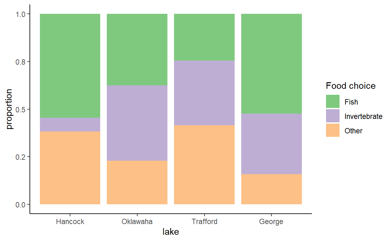
What proportion of alligators from Lake Hancock had invertebrates as their main food choice? How does this proportion compare to the other three lakes?
From the proportions table above: 7%.
Now fit a multinomial logistic regression model for food choice against lake.
lake_model <- multinom(food ~ lake, data = alligators,
                       trace = FALSE) # hide output
summary(lake_model)
Call:
multinom(formula = food ~ lake, data = alligators, trace = FALSE)

Coefficients:
             (Intercept) lakeOklawaha lakeTrafford lakeGeorge
Invertebrate        -2.0            2          2.3        1.5
Reptile             -2.3            1          1.8       -1.2
Bird                -1.8           -1          0.6       -0.6
Other               -0.8           -1          0.6       -0.9

Std. Errors:
             (Intercept) lakeOklawaha lakeTrafford lakeGeorge
Invertebrate         0.5          0.6          0.6        0.6
Reptile              0.6          0.8          0.8        1.2
Bird                 0.5          1.1          0.7        0.8
Other                0.3          0.7          0.5        0.6

Residual Deviance: 561
AIC: 593
This particular summary doesn’t give a \(\chi^2\) statistic but you can compute one yourself. Does this suggest that the primary food differs between the lakes?
with(alligators, chisq.test(food, lake))
    Pearson's Chi-squared test

data:  food and lake
X-squared = 38, df = 12, p-value = 2e-04
What is the odds ratio for preferring invertebrates to fish in lake Oklawaha compared to Lake Hancock? Does this agree with what you saw in the table?
Fish and Lake Hancock are both reference levels in this case, so we can just read off the coefficients.
exp(coefficients(lake_model))['Invertebrate', 'lakeOklawaha']
[1] 8Confirm your answer to the previous question by using a single logistic regression model.
lake_model2 <- glm(food == 'Invertebrate' ~ lake,
                   data = alligators,
                   subset = food %in% c('Invertebrate', 'Fish'),
                   family = binomial)

exp(coefficients(lake_model2))['lakeOklawaha']
lakeOklawaha
           8
Using nnet::multinom
This section uses the dataset politics.dta which contains information on the effect of gender and race on political party identification in the United States.
Use levels to find out the meanings of the variables.
lapply(politics, levels)
$gender
[1] "Male"   "Female"

$race
[1] "White" "Black"

$party
[1] "Democrat"    "Republican"  "Independent"
Use a multinomial model to determine the effect of race on party affiliation. How does being black affect the odds of being a Republican rather than a Democrat?
library(nnet)
party_model <- multinom(party ~ race, data = politics,
                        trace = FALSE)
exp(coefficients(party_model))
            (Intercept) raceBlack
Republican          1.0       0.1
Independent         0.8       0.3
Black people are less likely to be Republicans versus Democrats; the odds ratio is 0.1.
Note. “White” and “Democrat” are both reference levels in this model.
How does being black affect the odds of being an independent rather than a Democrat?
From the output above, the odds ratio of being an independent rather than a Democrat is 0.3 for those people identified as black.
Use table or xtabs to check whether your answers to the previous questions are sensible.
xtabs(~ party + race, data = politics)
             race
party         White Black
  Democrat      304    98
  Republican    305    10
  Independent   257    27
What is the odds ratio for being a Republican rather than a Democrat for women compared to men?
party_model2 <- multinom(party ~ gender, data = politics, trace = FALSE)
exp(coefficients(party_model2))
            (Intercept) genderFemale
Republican          1.0          0.6
Independent         0.8          0.8
The odds ratio is 0.6.
Verify this with a logistic regression model. (Here we column-bind the parameter estimates with their 95% confidence intervals.)
party_model3 <- glm(party == 'Republican' ~ gender,
                    data = politics,
                    subset = party != 'Independent',
                    family = binomial)

exp(
  cbind(estimate = coefficients(party_model3),
        confint(party_model3))
)
             estimate 2.5 % 97.5 %
(Intercept)       1.0   0.8    1.3
genderFemale      0.6   0.4    0.8
Fit a multinomial model in which party identification is predicted from both race and gender.
party_model4 <- multinom(party ~ race + gender, data = politics)
Add the interaction between race and gender, to see if the race influence differs between men and women. Is this difference statistically significant?
Either fit the model again with another call to multinom, or add the term to the model using update:
party_model5 <- update(party_model4, . ~ . + race:gender)
Compare the two models with a \(\chi^2\) test:
anova(party_model5, party_model4)
| Model | Resid. df | Resid. Dev | Test | Df | LR stat. | Pr(Chi) |
|---|---|---|---|---|---|---|
| race + gender | 1996 | 2086 | ||||
| race + gender + race:gender | 1994 | 2086 | 1 vs 2 | 2 | 0.2 | 0.9 |
The difference is not statistically significant, implying the influence of race is not different for men versus women.
Ordinal models
Ordered logistic/probit regression models are implemented by the polr function from the MASS (Modern Applied Statistics with S) package.
This section uses the data in housing.dta. These data concern levels of satisfaction among tenants of different types of housing, according how much contact they have with other residents and how much influence they feel they have over the management of their housing.
housing <- foreign::read.dta('http://personalpages.manchester.ac.uk/staff/mark.lunt/stats/8_Categorical/data/housing.dta')
Use levels to inspect the different factor levels.
lapply(housing, levels)
$contact
NULL

$satisfaction
[1] "Low"    "Medium" "High"

$housing
[1] "Tower Block"    "Apartment"      "Atrium House"
[4] "Terraced House"

$influence
[1] "Low"    "Medium" "High"

$`_Ihousing_2`
NULL

$`_Ihousing_3`
NULL

$`_Ihousing_4`
NULL
Does the degree of satisfaction depend on which type of housing the tenant lives in? (Use MASS::polr)
library(MASS)
housing_model <- polr(satisfaction ~ housing, data = housing,
                      method = 'logistic')
summary(housing_model)
Call:
polr(formula = satisfaction ~ housing, data = housing, method = "logistic")

Coefficients:
                       Value Std. Error t value
housingApartment      -0.521      0.117   -4.47
housingAtrium House   -0.281      0.150   -1.87
housingTerraced House -1.057      0.148   -7.16

Intercepts:
            Value  Std. Error t value
Low|Medium  -1e+00  1e-01     -1e+01
Medium|High  7e-03  1e-01      7e-02

Residual Deviance: 3559.74
AIC: 3569.74
With which type of housing are the tenants most satisfied?
From the output above, all terms are negative, the reference level (tower blocks) have the most satisfied tenants.
Test whether influence and contact are significant predictors of satisfaction.
housing_model2 <- polr(satisfaction ~ influence + contact, data = housing,
                       method = 'logistic')
summary(housing_model2)
Call:
polr(formula = satisfaction ~ influence + contact, data = housing,
    method = "logistic")

Coefficients:
                Value Std. Error t value
influenceMedium 0.525     0.1044    5.03
influenceHigh   1.286     0.1258   10.22
contact         0.232     0.0937    2.47

Intercepts:
            Value Std. Error t value
Low|Medium  -0.06  0.10      -0.62
Medium|High  1.10  0.10      10.95

Residual Deviance: 3504.08
AIC: 3514.08 2.5 % 97.5 %
influenceMedium 1 2
influenceHigh 3 5
contact 1 2Confidence intervals for the odds ratios do not contain 1 (and for the log-odds do not contain 0), suggesting that the predictors are significant at the 5% level.
Create a multivariate model for predicting satisfaction from all of the variables that were significant univariately. Are these predictors all independently significant?
housing_model3 <- polr(satisfaction ~ housing + influence + contact,
                       data = housing, method = 'logistic')
exp(confint(housing_model3))
                      2.5 % 97.5 %
housingApartment        0.4    0.7
housingAtrium House     0.5    0.9
housingTerraced House   0.3    0.5
influenceMedium         1.4    2.0
influenceHigh           2.8    4.7
contact                 1.1    1.7
None of these confidence intervals of odds contains 1, implying all are significant.
Does the effect of influence depend on which type of housing a subject lives in? (i.e. is the influence:housing interaction significant?)
housing_model4 <- polr(satisfaction ~ housing * influence, data = housing,
                       method = 'logistic')
housing_model5 <- update(housing_model4, . ~ . - housing:influence)
anova(housing_model5, housing_model4)
Likelihood ratio tests of ordinal regression models

Response: satisfaction
                Model Resid. df Resid. Dev   Test    Df LR stat.
1 housing + influence      1656       3458
2 housing * influence      1650       3439 1 vs 2     6       19
  Pr(Chi)
1
2   0.004
The \(\chi^2\) test statistic is significant at the 5% level, implying there is an interaction effect.