David Selby: Lecture 3: Sampling and Confidence Intervals

This worksheet is based on the third lecture of the Statistical Modelling in Stata course, offered by the Centre for Epidemiology Versus Arthritis at the University of Manchester. The original Stata exercises and solutions are here translated into their R equivalents.

Refer to the original slides and Stata worksheets here.

Generating random samples

In this part of the practical, you are going to repeatedly generate random samples of varying size from a population with known mean and standard deviation. You can then see for yourselves how changing the sample size affects the variability of the sample mean.

Start a new R session.

In RStudio: go to Session > New Session, or clear the current working environment with Session > Clear Workspace….

In the original RGui, use Misc > Remove all objects.

Or in any console just type rm(list = ls()).

You could also create a new R Markdown document.

Create a variable called `n` that is equal to 5.

n <- 5

Draw a sample vector, `x`, of length `n` from a standard normal distribution.

The standard normal is a normal distribution with mean 0 and standard deviation 1. The rnorm command draws random normal samples of a specified size:

x <- rnorm(n, mean = 0, sd = 1)

In fact, in R the default arguments for rnorm are mean = 0 and sd = 1, so we can implicitly draw from the standard normal distribution with the more concise syntax:

x <- rnorm(n)

Calculate the sample mean of the vector `x`.

mean(x)

[1] -0.6742418

Equivalently,

sum(x) / length(x)

[1] -0.6742418

sum(x) / n

[1] -0.6742418

Repeat steps 1–4 ten times and record the results as the first column of a data frame called `sample_means`.

You can save yourself from mashing the same command in multiple times, and in any case you should never enter data in manually if you can avoid it. You can repeat a non-deterministic function using the function replicate. So to draw the ten samples, we could write

replicate(10, rnorm(n))

            [,1]       [,2]      [,3]       [,4]       [,5]
[1,]  0.06945952 -1.2103535 -1.556742 -0.6525782  1.1921979
[2,] -0.13776090  0.9531469 -1.639101  0.1003915  0.6924461
[3,]  0.63740557 -1.9423815 -1.091731  1.4434986  1.9045813
[4,]  1.46863079  0.5541021  1.461920 -0.1230688 -0.2513096
[5,] -0.12372720 -0.7676365  1.087870 -0.7365115 -0.6336294
           [,6]       [,7]       [,8]       [,9]      [,10]
[1,]  0.1121903 -0.7122230  0.2062728 -1.1138570  0.5896345
[2,] -1.3490356 -1.0788139  0.6951568 -0.5759782 -0.5696374
[3,]  0.2582184 -0.2540282 -0.8108937 -0.9925909  1.2790741
[4,] -0.1198645  1.1782292  2.9030912  0.5917757 -0.9614041
[5,]  0.4952502  1.3589558 -0.7183756  1.5438060 -1.0640794

But we are only interested in the ten means rather than all 50 individual values, so sample and summarise in a single step by typing

replicate(10, mean(rnorm(n)))

 [1]  0.66612788 -0.01143214  0.29008491 -0.56442805 -0.29847374
 [6]  0.41514008  0.28023506  0.23828527 -0.14311970  0.20587570

To store such a vector as a column called n_5 in a new data frame, we can run

sample_means <- data.frame(n_5 = replicate(10, mean(rnorm(n))))

Of course, you can name the columns whatever you like.

Now repeat the procedure a further ten times, but in step 2, set the sample size to 25. Store the result.

An efficient way to tackle this task could be to run code similar to the following:

n <- 25
sample_means$n_25 <- replicate(10, mean(rnorm(n)))

Add a third column to your data frame corresponding to the means of ten vectors of sample size `n` = 100.

As before:

n <- 100
sample_means$n_100 <- replicate(10, mean(rnorm(n)))

The resulting data frame might look something like:

sample_means

           n_5         n_25        n_100
1  -0.17915405  0.124004806 -0.197642952
2  -0.35920449 -0.043915086 -0.169110213
3   0.09009174  0.026120982  0.038052114
4   0.55404695 -0.008663792 -0.109587922
5   0.93139574 -0.292556345  0.005135721
6  -0.25395434 -0.044169942 -0.069154800
7   0.38099651  0.122210811 -0.210156547
8   0.82132940 -0.141029992  0.084430420
9   0.40604792  0.015085206 -0.033767801
10  0.31336382  0.017653344 -0.065569055

Optional. If you consider yourself to be an annoying over-achiever, you can complete all of the above tasks with a single command, for example

sample_means <- as.data.frame(
  sapply(c(5, 25, 100),
         function(n) replicate(10, mean(rnorm(n))))
)

Optional. Furthermore, savvy statisticians might recognise that the sample mean of a normally distributed random variable has distribution \[\hat\mu \sim N(0, \sigma^2/n) \] so you can sample the means directly rather than generating the varying-length vectors.

sample_means <- data.frame(
  n_5   = rnorm(10, sd = 1 / sqrt(5)),
  n_25  = rnorm(10, sd = 1 / sqrt(25)),
  n_100 = rnorm(10, sd = 1 / sqrt(100))
)

Now calculate the mean and standard deviation of the values in each column.

Everything is in a data frame, so finding summary statistics for each column is straightforward. For each column, we can call something like

mean(sample_means$n_5)

[1] 0.2704959

sd(sample_means$n_5)

[1] 0.4421326

But to save time typing that out three times, we can calculate for all the columns at once:

apply(sample_means, MARGIN = 2, FUN = mean)

       n_5       n_25      n_100 
 0.2704959 -0.0225260 -0.0727371

apply(sample_means, MARGIN = 2, FUN = sd)

       n_5       n_25      n_100 
0.44213260 0.12287900 0.09986336

where the second argument, 2, means we are calculating the means of the second dimension (the columns), rather than of the first dimension (the rows) of our data frame.

A shorthand for calculating the means is:

colMeans(sample_means)

       n_5       n_25      n_100 
 0.2704959 -0.0225260 -0.0727371

and while there isn’t a function called colVars or colSDs, you can compute the variance–covariance matrix and read the numbers off the diagonal:

cov(sample_means)

              n_5         n_25        n_100
n_5    0.19548123 -0.029648661  0.023664380
n_25  -0.02964866  0.015099248 -0.007692111
n_100  0.02366438 -0.007692111  0.009972690

# Just the diagonal entries
sqrt(diag(cov(sample_means)))

       n_5       n_25      n_100 
0.44213260 0.12287900 0.09986336

If you prefer dplyr:

library(dplyr)
summarise_all(sample_means, mean)

        n_5      n_25      n_100
1 0.2704959 -0.022526 -0.0727371

summarise_all(sample_means, sd)

        n_5     n_25      n_100
1 0.4421326 0.122879 0.09986336

And finally data.table:

library(data.table)
setDT(sample_means)
sample_means[, .(n = names(sample_means),
                 mean = sapply(.SD, mean),
                 sd = sapply(.SD, sd))]

       n       mean         sd
1:   n_5  0.2704959 0.44213260
2:  n_25 -0.0225260 0.12287900
3: n_100 -0.0727371 0.09986336

Means

This section is bookwork and does not require R or Stata.

If the standard deviation of the original distribution is \(\sigma\), then the standard error of the sample mean is \(\sigma/\sqrt{n}\), where \(n\) is the sample size.

If the standard deviation of measured heights is 9.31 cm, what will be the standard error of the mean in:
1. a sample of size 49?
2. a sample of size 100?
Imagine we only had data on a sample of size 100, where the sample mean was 166.2 cm and the sample standard deviation was 10.1 cm.
1. Calculate the standard error for this sample mean (using the sample standard deviation as an estimate of the population standard deviation).
2. Calculate the interval ranging 1.96 standard errors either side of the sample mean.
Imagine we only had data on a sample size of 36 where the sample mean height was 163.5 cm and the standard deviation was 10.5cm.
1. Within what interval would you expect about 95% of heights from this population to lie (the reference range)?
2. Calculate the 95% confidence interval for the sample mean.
Figure 1 is a histogram of measured weight in a sample of 100 individuals.
1. Would it be better to use the mean and standard deviation or the median and interquartile range to summarise these data?
2. If the mean of the data is 69.69 kg with a standard deviation of 12.76 kg, calculate a 95% confidence interval for the mean.
3. Why is it not sensible to calculate a 95% reference range for these data?

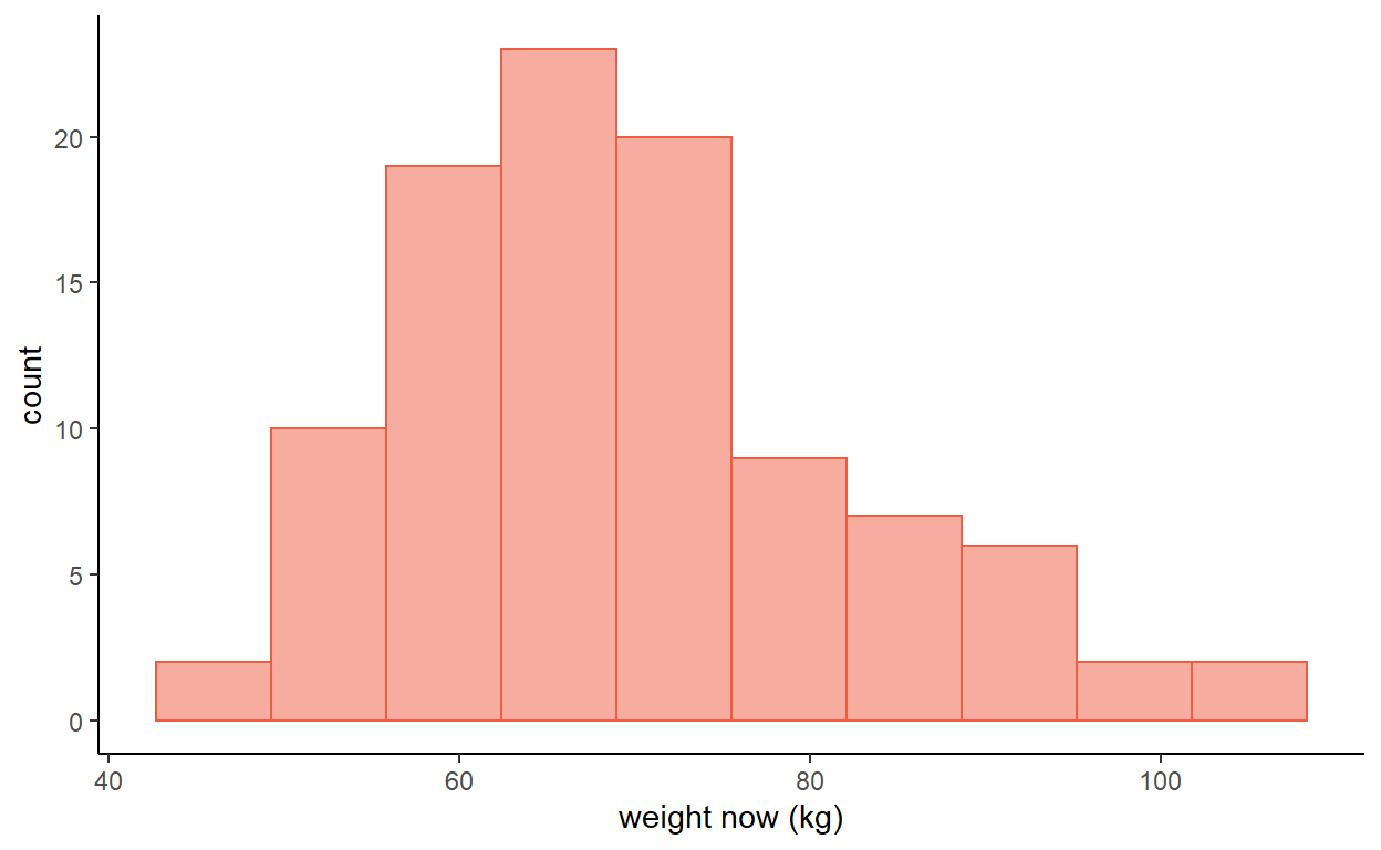
Figure 1: Weights in a random sample of 100 women

Proportions

This section is bookwork and does not require R or Stata.

Again using our height and weight dataset of 412 individuals, 234 (56.8%) are women and 178 (43.2%) are men.

If we take a number of smaller samples from this population, the proportion of women will vary, although they will tend to be scattered around 57%. Figure 2 represents 50 samples, each of size 40.

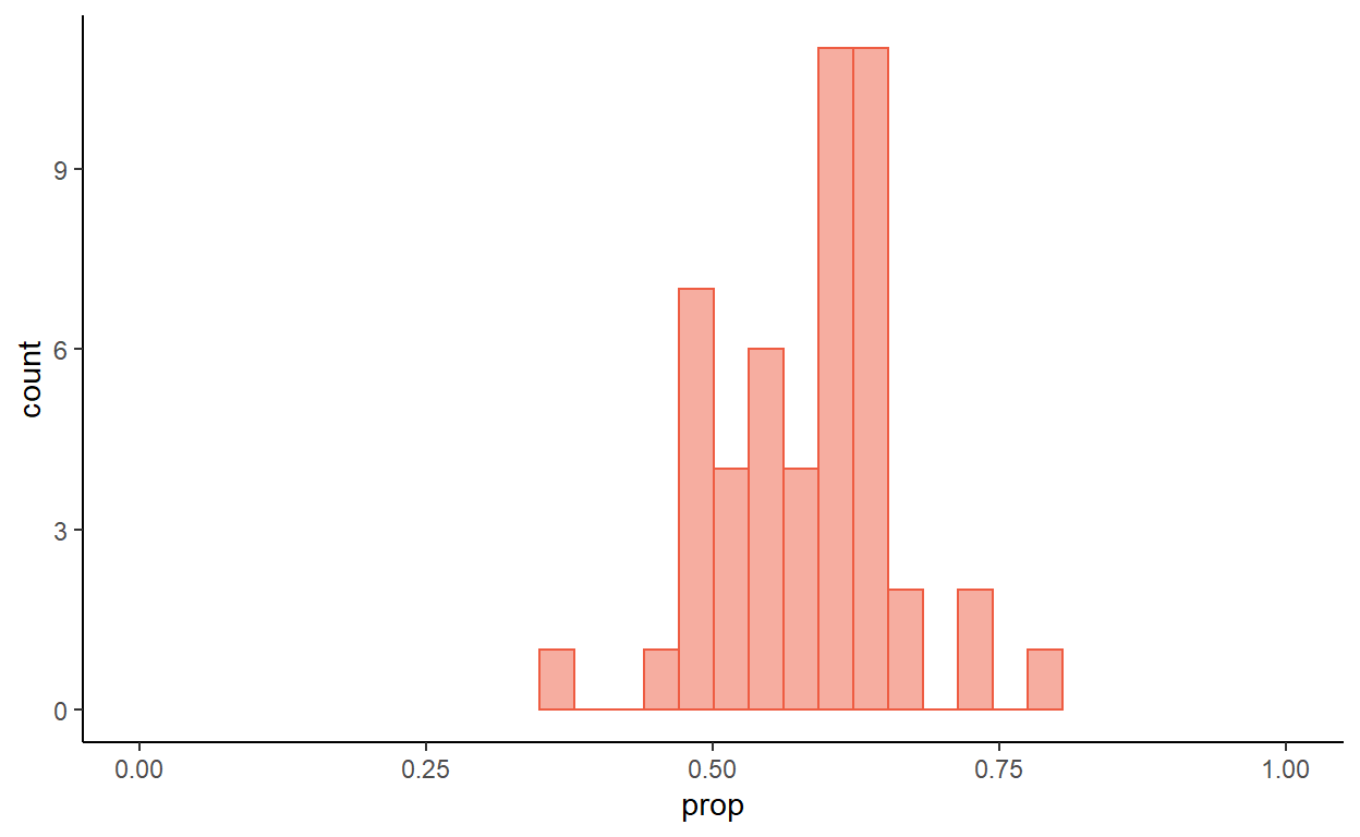
Figure 2: Proportion of women in 50 samples of size 40

What would you expect to happen if the sample sizes were bigger, say \(n=100\)?
In a sample of 40 individuals from a larger population, 25 are women. Calculate a 95% confidence interval for the proportion of women in the population.

Note. When sample sizes are small, the use of standard errors and the normal distribution does not work well for proportions. This is only really a problem if \(p\) (or \((1-p)\)) is less than \(5/n\) (i.e. there are fewer than 5 subjects in one of the groups).

From a random sample of 80 women who attend a general practice, 18 report a previous history of asthma.
1. Estimate the proportion of women in this population with a previous history of asthma, along with a 95% confidence interval for this proportion.
2. Is the use of the normal distribution valid in this instance?
In a random sample of 150 Manchester adults it was found that 58 received or needed to receive treatment for defective vision. Estimate:
1. the proportion of adults in Manchester who receive or need to receive treatment for defective vision,
2. a 95% confidence interval for this proportion.

Confidence intervals in R

Download the bpwide.csv dataset.

Load the blood pressure data in its wide form into R with the command

bpwide <- read.csv('bpwide.csv')

This is fictional data concerning blood pressure before and after a particular intervention.

Use an appropriate visualisation to see if the variable `bp_before` is normally distributed. What do you think?

The original Stata solution calls for a histogram, for example:

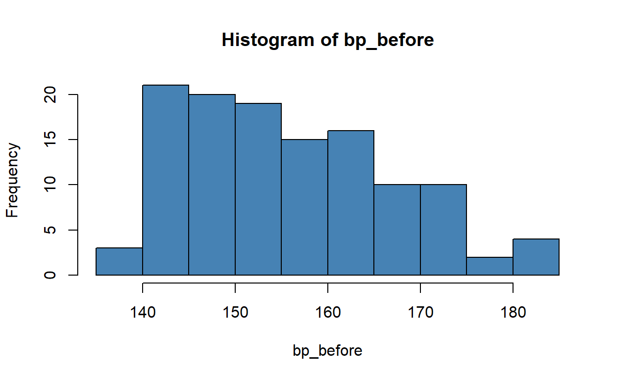
with(bpwide, hist(bp_before, col = 'steelblue'))

However, a kernel density plot may be a slightly better way of visualising the distribution.

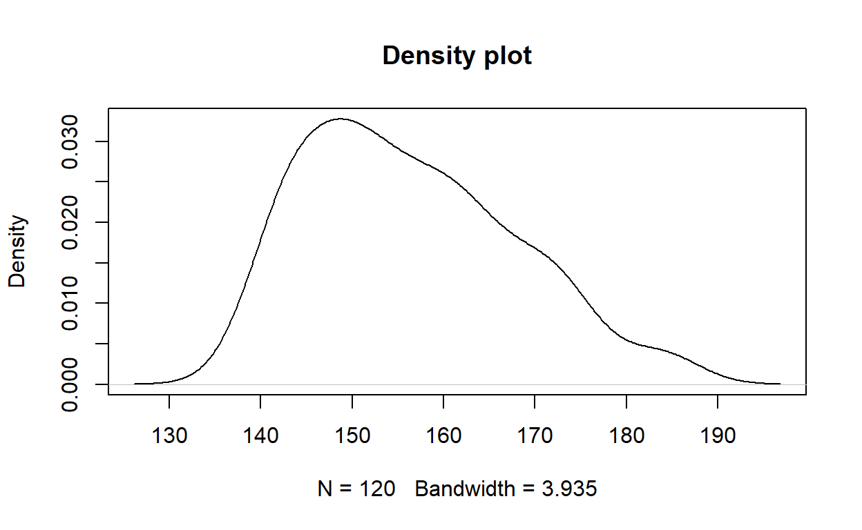
plot(density(bpwide$bp_before), main = 'Density plot')

The question, however, asked for “an appropriate visualisation” to determine if the variable is normally distributed. You might like to think that you can tell if a curve is bell-shaped, but this is not a reliable way of answering the question. A more appropriate visualisation is a quantile–quantile plot, where we can compare the sample quantiles of the observed data with the theoretical quantiles of a normal distribution.

Now you don’t need to remember the ideal shape of a bell curve—just look at the points and see if they lie close to the line or not.

qqnorm(bpwide$bp_before)
qqline(bpwide$bp_before)

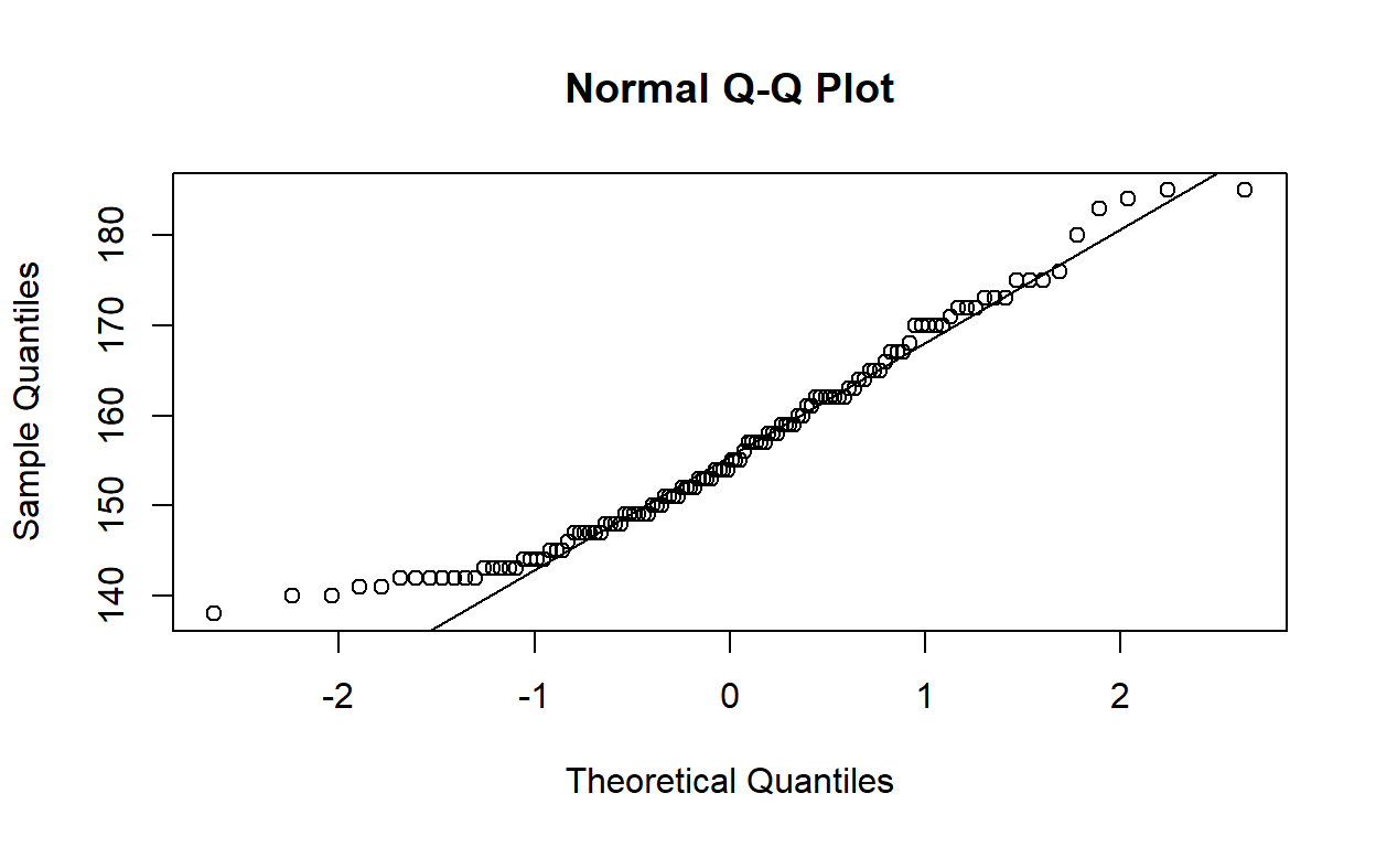
There is a slight positive (right) skew.

Create a new variable to measure the change in blood pressure.

You can create a standalone variable:

bp_diff <- with(bpwide, bp_after - bp_before)

Or, since it is of the same length as bp_after and bp_before, you can store it as a new column in the bpwide data frame.

bpwide <- transform(bpwide, bp_diff = bp_after - bp_before)

What is the mean change in blood pressure?

mean(bp_diff)

[1] -5.091667

mean(bpwide$bp_diff)

[1] -5.091667

Compute a confidence interval for the change in blood pressure.

As we are looking at a difference in means, we compare the sample blood pressure difference to a Student’s t distribution with \(n - 1\) degrees of freedom, where \(n\) is the number of patients.

By hand: the formula for a two-sided \((1-\alpha)\) confidence interval for a sample of size \(n\) is \[Pr\left(\bar{X}_n - t_{n-1}(\alpha/2) \frac{S_n}{\sqrt n} < \mu < \bar{X} + t_{n-1}(\alpha/2) \frac{S_n}{\sqrt n}\right) = \alpha \]

In R, the q family of functions returns quantiles of distributions (just as we have seen the r family draws random samples from those distributions). So qnorm finds the quantiles of the normal distribution, qt the quantiles of the Student’s t-distribution, and so on. We can use it to retrieve the 2.5% and 97.5% quantiles of the t distribution with \(n-1\) degrees of freedom and then plug them into the above formula, like so:

n <- length(bp_diff) # or nrow(bpwide)
mean(bp_diff) + qt(c(.025, .975), df = n - 1) * sd(bp_diff) / sqrt(n)

[1] -8.112776 -2.070557

Or, using the built-in t.test function we get the same result:

with(bpwide, t.test(bp_before, bp_after, paired = TRUE))


    Paired t-test

data:  bp_before and bp_after
t = 3.3372, df = 119, p-value = 0.00113
alternative hypothesis: true difference in means is not equal to 0
95 percent confidence interval:
 2.070557 8.112776
sample estimates:
mean of the differences 
               5.091667

As the 95% confidence interval does not contain zero, we may reject the hypothesis that, on average, there was no change in blood pressure.

Notice that the paired t.test did not require us to calculate bp_diff. But we can pass the same to t.test for a one-sample test and it will compute exactly the same test statistic, because testing whether two variables are equal is the same thing as testing whether their paired difference is zero.

t.test(bp_diff)


    One Sample t-test

data:  bp_diff
t = -3.3372, df = 119, p-value = 0.00113
alternative hypothesis: true mean is not equal to 0
95 percent confidence interval:
 -8.112776 -2.070557
sample estimates:
mean of x 
-5.091667

Look at the histogram of changes in blood pressure using the command `hist`.

hist(bp_diff, col = 'steelblue')

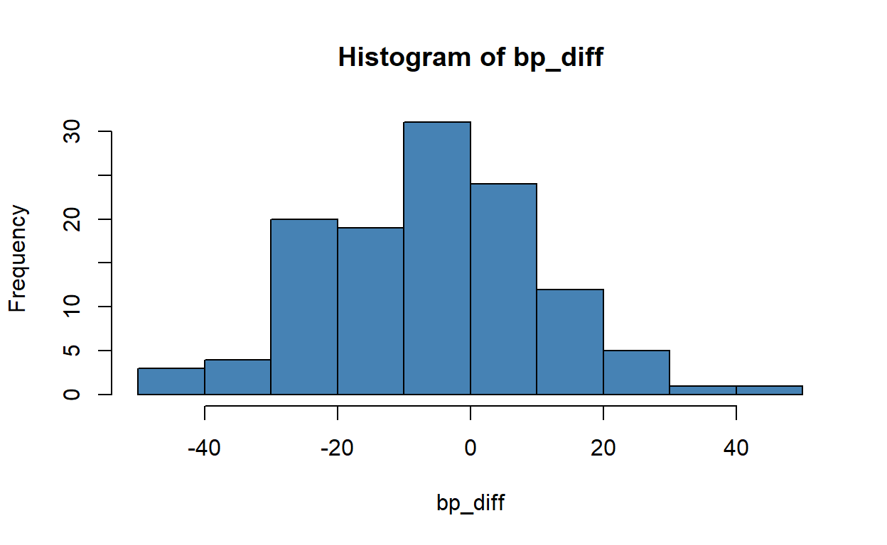
You could also try a kernel density plot, or even an old-fashioned stem and leaf diagram:

stem(bp_diff)


  The decimal point is 1 digit(s) to the right of the |

  -4 | 55
  -4 | 2
  -3 | 
  -3 | 3000
  -2 | 99977776
  -2 | 443322222100
  -1 | 9988666555
  -1 | 422211000
  -0 | 9998877776655
  -0 | 43333333222111
   0 | 000022222333
   0 | 566777788899
   1 | 00001234444
   1 | 55599
   2 | 1
   2 | 5679
   3 | 
   3 | 6
   4 | 1

Does this confirm your answer to the previous question?

Create a new variable to indicate whether blood pressure went up or down in a given subject.

down <- with(bpwide, bp_after < bp_before)

Use the table command to see how many subjects showed a decrease in blood pressure.

table(down)

down
FALSE  TRUE 
   47    73

To get proportions, you can use prop.table, like so:

prop.table(table(down))

down
    FALSE      TRUE 
0.3916667 0.6083333

But it is just as quick to take the mean of the binary indicators (as TRUE == 1 and FALSE == 0):

mean(down)

[1] 0.6083333

mean(!down) # negation

[1] 0.3916667

Create a confidence interval for the proportion of subjects showing a decrease in blood pressure.

Note. This would rarely be justified. It is a good way to throw away a lot of continuous data, ignoring effect sizes. Moreover, one can easily flip the apparent sign of the effect by doing this, and draw the wrong conclusion about the data.

Nonetheless, if the purpose of the exercise is to make a Clopper–Pearson binomial confidence interval (as Stata does), then we have:

binom.test(sum(down), n)


    Exact binomial test

data:  sum(down) and n
number of successes = 73, number of trials = 120, p-value =
0.02208
alternative hypothesis: true probability of success is not equal to 0.5
95 percent confidence interval:
 0.5150437 0.6961433
sample estimates:
probability of success 
             0.6083333

Lecture 3: Sampling and Confidence Intervals