Bayesian modelling with Stan

Introduction to Stan, rstan and brms for multi-level Bayesian regession modelling.

Resources

1. View the talk slides (source code)
2. Stan web site
3. JAGS (Just Another Gibbs Sampler)
4. Statistical Rethinking book by Richard McElreath
5. Sleep deprivation study
   • original paper
   • access the dataset in R with data(sleepstudy, package = 'lme4')
6. brms: Bayesian regression modelling with Stan

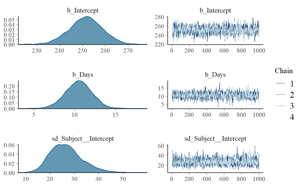
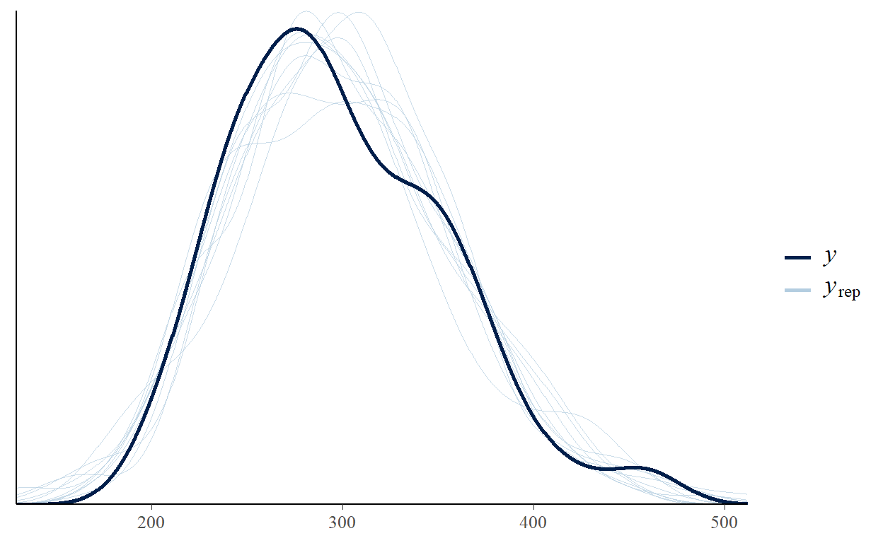
Final linear mixed model

fit <- brm(Reaction ~ Days + (Days | Subject),
           data = lme4::sleepstudy)

 Family: gaussian 
  Links: mu = identity; sigma = identity 
Formula: Reaction ~ Days + (Days | Subject) 
   Data: lme4::sleepstudy (Number of observations: 180) 
Samples: 4 chains, each with iter = 2000; warmup = 1000; thin = 1;
         total post-warmup samples = 4000

Group-Level Effects: 
~Subject (Number of levels: 18) 
                    Estimate Est.Error l-95% CI u-95% CI Rhat
sd(Intercept)          26.76      6.69    15.68    41.77 1.00
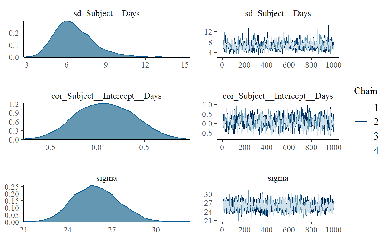
sd(Days)                6.58      1.51     4.22    10.11 1.00
cor(Intercept,Days)     0.09      0.30    -0.48     0.68 1.00
                    Bulk_ESS Tail_ESS
sd(Intercept)           2034     2769
sd(Days)                1635     1840
cor(Intercept,Days)      877     1633

Population-Level Effects: 
          Estimate Est.Error l-95% CI u-95% CI Rhat Bulk_ESS Tail_ESS
Intercept   251.45      7.45   236.65   265.67 1.00     1559     2236
Days         10.48      1.67     7.20    13.68 1.00     1385     2114

Family Specific Parameters: 
      Estimate Est.Error l-95% CI u-95% CI Rhat Bulk_ESS Tail_ESS
sigma    25.92      1.55    23.10    29.02 1.00     3193     2917

Samples were drawn using sampling(NUTS). For each parameter, Bulk_ESS
and Tail_ESS are effective sample size measures, and Rhat is the potential
scale reduction factor on split chains (at convergence, Rhat = 1).

plot(fit, N = 3)

pp_check(fit)