David Selby: Best practices for building baseline tables

Motivating examples

By James Gwinnutt and Stephanie Shoop-Worrall

Computing summary statistics with tidyverse

The iris dataset is built into R and gives the measured widths and lengths of sepals and petals for 150 examples of three different species of iris.

Let’s compute some ‘baseline’ summary statistics for these data using the package dplyr (part of the tidyverse family of packages).

For a single variable, such as the Petal.Length, we can calculate species-level statistics as follows.

data(iris)
library(tidyverse)
iris %>%
  group_by(Species) %>%
  summarise(mean = mean(Petal.Length),
            sd = sd(Petal.Length),
            n = n(),
            median = median(Petal.Length),
            Q1 = quantile(Petal.Length, .25),
            Q3 = quantile(Petal.Length, .75),
            IQR = IQR(Petal.Length),
            IQR1 = Q3 - Q1) # just another way of calculating iqr

# A tibble: 3 x 9
  Species     mean    sd     n median    Q1    Q3   IQR  IQR1
  <fct>      <dbl> <dbl> <int>  <dbl> <dbl> <dbl> <dbl> <dbl>
1 setosa      1.46 0.174    50   1.5    1.4  1.58 0.175 0.175
2 versicolor  4.26 0.470    50   4.35   4    4.6  0.600 0.600
3 virginica   5.55 0.552    50   5.55   5.1  5.88 0.775 0.775

If we want to compute the same summaries for the other variables: petal width, sepal width and sepal length, then we could just repeat the code above, swapping the name Petal.Length each time. But there is a better, less repetitive way.

Using another tidyverse package called tidyr, we can reshape the dataset into a long (rather than wide) table.

(iris_long <- iris %>%
  pivot_longer(-Species))

# A tibble: 600 x 3
   Species name         value
   <fct>   <chr>        <dbl>
 1 setosa  Sepal.Length   5.1
 2 setosa  Sepal.Width    3.5
 3 setosa  Petal.Length   1.4
 4 setosa  Petal.Width    0.2
 5 setosa  Sepal.Length   4.9
 6 setosa  Sepal.Width    3  
 7 setosa  Petal.Length   1.4
 8 setosa  Petal.Width    0.2
 9 setosa  Sepal.Length   4.7
10 setosa  Sepal.Width    3.2
# ... with 590 more rows

Instead of a separate column for each type of measurement, we have one column for the variable names and one for the values. Then the name can be just another group to pass to group_by:

iris_long %>%
  group_by(Species, Variable = name) %>%
  summarise(mean = mean(value),
            sd = sd(value),
            n = n(),
            median = median(value),
            Q1 = quantile(value, .25),
            Q3 = quantile(value, .75),
            IQR = IQR(value))

# A tibble: 12 x 9
# Groups:   Species [3]
   Species    Variable      mean    sd     n median    Q1    Q3   IQR
   <fct>      <chr>        <dbl> <dbl> <int>  <dbl> <dbl> <dbl> <dbl>
 1 setosa     Petal.Length 1.46  0.174    50   1.5   1.4   1.58 0.175
 2 setosa     Petal.Width  0.246 0.105    50   0.2   0.2   0.3  0.100
 3 setosa     Sepal.Length 5.01  0.352    50   5     4.8   5.2  0.4  
 4 setosa     Sepal.Width  3.43  0.379    50   3.4   3.2   3.68 0.475
 5 versicolor Petal.Length 4.26  0.470    50   4.35  4     4.6  0.600
 6 versicolor Petal.Width  1.33  0.198    50   1.3   1.2   1.5  0.3  
 7 versicolor Sepal.Length 5.94  0.516    50   5.9   5.6   6.3  0.7  
 8 versicolor Sepal.Width  2.77  0.314    50   2.8   2.52  3    0.475
 9 virginica  Petal.Length 5.55  0.552    50   5.55  5.1   5.88 0.775
10 virginica  Petal.Width  2.03  0.275    50   2     1.8   2.3  0.500
11 virginica  Sepal.Length 6.59  0.636    50   6.5   6.22  6.9  0.675
12 virginica  Sepal.Width  2.97  0.322    50   3     2.8   3.18 0.375

From here, see the last section on how we might turn this into a publication-quality table like below.

	Mean	SD	Median	Q1	Q3	IQR
setosa (N = 50)
Petal Length	1.5	0.2	1.5	1.4	1.6	0.2
Petal Width	0.2	0.1	0.2	0.2	0.3	0.1
Sepal Length	5.0	0.4	5.0	4.8	5.2	0.4
Sepal Width	3.4	0.4	3.4	3.2	3.7	0.5
versicolor (N = 50)
Petal Length	4.3	0.5	4.3	4.0	4.6	0.6
Petal Width	1.3	0.2	1.3	1.2	1.5	0.3
Sepal Length	5.9	0.5	5.9	5.6	6.3	0.7
Sepal Width	2.8	0.3	2.8	2.5	3.0	0.5
virginica (N = 50)
Petal Length	5.6	0.6	5.6	5.1	5.9	0.8
Petal Width	2.0	0.3	2.0	1.8	2.3	0.5
Sepal Length	6.6	0.6	6.5	6.2	6.9	0.7
Sepal Width	3.0	0.3	3.0	2.8	3.2	0.4

Recoding variables

Sometimes variables aren’t quite in the data type that we want. For example, we might want to split a continuous variable like BMI into categories based on pre-specified cutpoints. Suppose our vector of BMIs was

bmi <- c(29.4, 11.4, 24.5, 19.1, -0.6, 7.9, NA, 20.1, 30, 40.9)

And the pre-specified groups boundaries are at 0, 18.5, 25, 30, 35 and 40. One way of doing this would be a series of nested ifelse() expressions.

ifelse(bmi >= 0 & bmi < 18.5, '[0, 18.5)',
       ifelse(bmi >= 18.5 & bmi < 25, '[18.5, 25)',
              ifelse(bmi >= 25 & bmi < 30, '[25, 30)',
                     ifelse(bmi >= 30 & bmi < 35, '[30, 35)',
                            ifelse(bmi >= 35 & bmi < 40, '[35, 40)',
                                   ifelse(bmi >= 40, '40+', NA))))))

 [1] "[25, 30)"   "[0, 18.5)"  "[18.5, 25)" "[18.5, 25)" NA          
 [6] "[0, 18.5)"  NA           "[18.5, 25)" "[30, 35)"   "40+"

However, this is tedious to write, error-prone and unnecessarily verbose. There are built-in functions to do this! One is called cut() and the other is called findInterval(). The former creates a factor variable, labelled according to the interval in which each value falls. The latter is similar but just returns an integer corresponding to the interval.

cutpoints <- c(0, 18.5, 25, 30, 35, 40)
cut(bmi, cutpoints)

 [1] (25,30]   (0,18.5]  (18.5,25] (18.5,25] <NA>      (0,18.5] 
 [7] <NA>      (18.5,25] (25,30]   <NA>     
Levels: (0,18.5] (18.5,25] (25,30] (30,35] (35,40]

By default, anything greater than the last cutpoint (or smaller than the first), if passed to cut(), is categorised as NA. To avoid this happening, you can set the first and last cutpoints to arbitrarily small and high numbers, respectively (such as -Inf and +Inf).

Negative BMIs are clearly invalid but let’s try to keep the 40+ ones. To match the first example, let’s also have the intervals open (exclusive) on the right:

cut(bmi, c(cutpoints, Inf), right = FALSE)

 [1] [25,30)   [0,18.5)  [18.5,25) [18.5,25) <NA>      [0,18.5) 
 [7] <NA>      [18.5,25) [30,35)   [40,Inf) 
Levels: [0,18.5) [18.5,25) [25,30) [30,35) [35,40) [40,Inf)

Alternatively, the related function findInterval() will classify anything before the first cutpoint as group 0 and anything after the last cutpoint as group \(n_\text{cutpoints}+1\).

findInterval(bmi, cutpoints)

 [1]  3  1  2  2  0  1 NA  2  4  6

Explore the documentation for both functions to see what other options are available.

Now let’s use what we’ve learnt to count the number of patients in each group. Suppose the data are stored in a data frame called bmi_data:

Then a dplyr approach might be

bmi_data %>%
  mutate(bmi_group = findInterval(bmi, cutpoints)) %>%
  count(bmi_group)

  bmi_group n
1         0 1
2         1 2
3         2 3
4         3 1
5         4 1
6         6 1
7        NA 1

Here’s a base R solution, using automatic labels and treating negative BMIs as invalid.

bmi_data <- transform(bmi_data,
                      bmi_group = cut(bmi, c(cutpoints, Inf)))

table(bmi_data$bmi_group)


 (0,18.5] (18.5,25]   (25,30]   (30,35]   (35,40]  (40,Inf] 
        2         3         2         0         0         1

table(bmi_data$bmi_group, useNA = 'ifany')


 (0,18.5] (18.5,25]   (25,30]   (30,35]   (35,40]  (40,Inf]      <NA> 
        2         3         2         0         0         1         2

Merging categories

Imagine we want to merge categories that have fewer than 10 people in them, for confidentiality purposes. There are many ways you might do this.

example_data

# A tibble: 500 x 3
      id country     score
   <int> <chr>       <dbl>
 1     1 Spain          14
 2     2 Ireland        17
 3     3 Montenegro     29
 4     4 Portugal       21
 5     5 Romania        25
 6     6 Latvia         13
 7     7 Isle of Man    23
 8     8 Guernsey       10
 9     9 Slovenia       21
10    10 Andorra        25
# ... with 490 more rows

One way is to add_counts for each group, then mutate using ifelse. Here I am creating a new column called new_country so you can compare them.

example_data %>%
  add_count(country, name = 'N') %>%
  mutate(new_country = ifelse(N < 10, 'Other', country))

# A tibble: 500 x 5
      id country     score     N new_country
   <int> <chr>       <dbl> <int> <chr>      
 1     1 Spain          14    16 Spain      
 2     2 Ireland        17    13 Ireland    
 3     3 Montenegro     29     7 Other      
 4     4 Portugal       21     7 Other      
 5     5 Romania        25    11 Romania    
 6     6 Latvia         13     9 Other      
 7     7 Isle of Man    23    11 Isle of Man
 8     8 Guernsey       10     8 Other      
 9     9 Slovenia       21    11 Slovenia   
10    10 Andorra        25    13 Andorra    
# ... with 490 more rows

Alternatively, you might use the fct_lump_min (factor lump) function from the forcats (“for categorical variables”) package, which is specifically designed for this sort of task. There are lots of other fun functions for manipulating categorical variables in that package; check it out!

example_data %>%
  mutate(new_country = forcats::fct_lump_min(country, min = 10))

# A tibble: 500 x 4
      id country     score new_country
   <int> <chr>       <dbl> <fct>      
 1     1 Spain          14 Spain      
 2     2 Ireland        17 Ireland    
 3     3 Montenegro     29 Other      
 4     4 Portugal       21 Other      
 5     5 Romania        25 Romania    
 6     6 Latvia         13 Other      
 7     7 Isle of Man    23 Isle of Man
 8     8 Guernsey       10 Other      
 9     9 Slovenia       21 Slovenia   
10    10 Andorra        25 Andorra    
# ... with 490 more rows

Or if you prefer data.table, this solution is analogous to using dplyr::add_count. The row-indexing syntax saves us a call to ifelse (or fifelse or if_else…).

library(data.table)
setDT(example_data)
example_data[, N := .N, by = country]
example_data[N < 10, country := 'Other']
example_data

      id country score  N
  1:   1   Spain    14 16
  2:   2 Ireland    17 13
  3:   3   Other    29  7
  4:   4   Other    21  7
  5:   5 Romania    25 11
 ---                     
496: 496   Other    26  8
497: 497   Other    17  7
498: 498   Other    33  7
499: 499   Other    23  8
500: 500 Albania    16 11

Counting missing values

How much missing data is there for each variable in the baseline table? Here’s an example using the airquality dataset (which is built into base R and contains some missing values).

data(airquality)
head(airquality)

  Ozone Solar.R Wind Temp Month Day
1    41     190  7.4   67     5   1
2    36     118  8.0   72     5   2
3    12     149 12.6   74     5   3
4    18     313 11.5   62     5   4
5    NA      NA 14.3   56     5   5
6    28      NA 14.9   66     5   6

The base summary function will report NA counts, if any.

summary(airquality)

     Ozone           Solar.R           Wind             Temp      
 Min.   :  1.00   Min.   :  7.0   Min.   : 1.700   Min.   :56.00  
 1st Qu.: 18.00   1st Qu.:115.8   1st Qu.: 7.400   1st Qu.:72.00  
 Median : 31.50   Median :205.0   Median : 9.700   Median :79.00  
 Mean   : 42.13   Mean   :185.9   Mean   : 9.958   Mean   :77.88  
 3rd Qu.: 63.25   3rd Qu.:258.8   3rd Qu.:11.500   3rd Qu.:85.00  
 Max.   :168.00   Max.   :334.0   Max.   :20.700   Max.   :97.00  
 NA's   :37       NA's   :7                                       
     Month            Day      
 Min.   :5.000   Min.   : 1.0  
 1st Qu.:6.000   1st Qu.: 8.0  
 Median :7.000   Median :16.0  
 Mean   :6.993   Mean   :15.8  
 3rd Qu.:8.000   3rd Qu.:23.0  
 Max.   :9.000   Max.   :31.0

Or you can loop over the columns and compute the counts and proportions:

airquality_nas <- airquality[, 1:4]
airquality_nas[] <- lapply(airquality_nas, is.na)
colSums(airquality_nas)

  Ozone Solar.R    Wind    Temp 
     37       7       0       0

100 * colMeans(airquality_nas)

    Ozone   Solar.R      Wind      Temp 
24.183007  4.575163  0.000000  0.000000

In dplyr, it might look something like this:

airquality %>%
  pivot_longer(Ozone:Temp) %>% # ignore Day & Month
  group_by(name) %>%
  summarise(total = n(),
            present = sum(!is.na(value)),
            missing = sum(is.na(value)),
            `% present` = 100 * present / total,  # or mean(!is.na(value))
            `% missing` = 100 * missing / total)  # or mean(is.na(value))

# A tibble: 4 x 6
  name    total present missing `% present` `% missing`
  <chr>   <int>   <int>   <int>       <dbl>       <dbl>
1 Ozone     153     116      37        75.8       24.2 
2 Solar.R   153     146       7        95.4        4.58
3 Temp      153     153       0       100          0   
4 Wind      153     153       0       100          0

And in data.table:

setDT(airquality)
airquality[, lapply(.SD, is.na)][,
                                 .(column = names(.SD),
                                   total = .N,
                                   missing = sapply(.SD, sum),
                                   `% missing` = sapply(.SD, mean),
                                   present = .N - sapply(.SD, sum),
                                   `% present` = 1 - sapply(.SD, mean))]

    column total missing  % missing present % present
1:   Ozone   153      37 0.24183007     116 0.7581699
2: Solar.R   153       7 0.04575163     146 0.9542484
3:    Wind   153       0 0.00000000     153 1.0000000
4:    Temp   153       0 0.00000000     153 1.0000000
5:   Month   153       0 0.00000000     153 1.0000000
6:     Day   153       0 0.00000000     153 1.0000000

The TableOne package

By Ruth Costello

The R package tableone quickly produces a table that is easy to use in medical research papers. Given a specification of variables (vars), factors (factorVars) and groups (strata), it computes common summary statistics automatically.

For example:

library(tableone)
CreateTableOne(
  vars = c('Petal.Length', 'Petal.Width'),
  strata = 'Species',
  data = iris
)

                          Stratified by Species
                           setosa      versicolor  virginica   p      test
  n                          50          50          50                   
  Petal.Length (mean (SD)) 1.46 (0.17) 4.26 (0.47) 5.55 (0.55) <0.001     
  Petal.Width (mean (SD))  0.25 (0.11) 1.33 (0.20) 2.03 (0.27) <0.001

Another example:

CreateTableOne(
  vars = c('age', 'sex', 'state', 'T.categ'),
  factorVars = c('state', 'sex', 'T.categ'),
  data = MASS::Aids2
)

                 
                  Overall      
  n                2843        
  age (mean (SD)) 37.41 (10.06)
  sex = M (%)      2754 (96.9) 
  state (%)                    
     NSW           1780 (62.6) 
     Other          249 ( 8.8) 
     QLD            226 ( 7.9) 
     VIC            588 (20.7) 
  T.categ (%)                  
     hs            2465 (86.7) 
     hsid            72 ( 2.5) 
     id              48 ( 1.7) 
     het             41 ( 1.4) 
     haem            46 ( 1.6) 
     blood           94 ( 3.3) 
     mother           7 ( 0.2) 
     other           70 ( 2.5)

Other, similar packages you might like try include:

Package TableOne (not on CRAN; based on this paper)
Package table1
Package gtsummary

Neater knitr tables

By David Selby

Generating tables by hand

If copying data from an external source (rather than calculating it yourself), then you might simply want to write in the data by hand. For this you can use a Markdown table, for instance, the following Markdown pipe table is copied from the supplementary materials of Dixon et al. (2019) and annotated with a Markdown caption.

Participants in the *Cloudy with a Chance of Pain* study (Dixon et al. 2019)
Variable	n	%
Number of participants	2658	100
Female	2210	83.1
Rheumatoid arthritis	506	19.0
Osteoarthritis	926	34.8
Ankylosing spondylitis	235	8.8
Gout	97	3.6
Arthritis (unspecified)	972	36.6
Fibromyalgia	665	25.0
Chronic headache	271	10.2
Neuropathic pain	371	14.0

using the following Markdown ‘pipe table’ syntax:

Table: Participants in the _Cloudy with a Chance of Pain_ study (Dixon et al, 2019)

| Variable                |    n |    % |
| :---------------------- | ---: | ---: |
| Number of participants  | 2658 |  100 |
| Female                  | 2210 | 83.1 |
| Rheumatoid arthritis    |  506 | 19.0 |
| Osteoarthritis          |  926 | 34.8 |
| Ankylosing spondylitis  |  235 |  8.8 |
| Gout                    |   97 |  3.6 |
| Arthritis (unspecified) |  972 | 36.6 |
| Fibromyalgia            |  665 | 25.0 |
| Chronic headache        |  271 | 10.2 |
| Neuropathic pain        |  371 | 14.0 |

But you don’t need to space the syntax perfectly. This works just as well:

Variable | n | %
:--- | ---: | ---:
Number of participants | 2658 |  100
Female | 2210 | 83.1
Rheumatoid arthritis |  506 | 19.0
Osteoarthritis |  926 | 34.8
Ankylosing spondylitis | 235 | 8.8
Gout | 97 |  3.6
Arthritis (unspecified) | 972 | 36.6
Fibromyalgia | 665 | 25.0
Chronic headache | 271 | 10.2
Neuropathic pain | 371 | 14.0

Which you can leave as-is, or you can neaten up automagically using the RStudio Addin Beautify Table from the beautifyR package. Install the addin from GitHub using the syntax

devtools::install_github('mwip/beautifyR')

then highlight your Markdown table and click Addins > Beautify Table from the toolbar.

Suppose you want to do some calculations with the copied data—not just display it in a table. You could enter it into a data frame by hand, using base syntax or the (slightly easier to read) tibble::tribble function:

my_tbl <- tibble::tribble(
                  ~Variable,    ~n, ~`%`,
   "Number of participants", 2658L,  100,
                   "Female", 2210L, 83.1,
     "Rheumatoid arthritis",  506L,   19,
           "Osteoarthritis",  926L, 34.8,
   "Ankylosing spondylitis",  235L,  8.8,
                     "Gout",   97L,  3.6,
  "Arthritis (unspecified)",  972L, 36.6,
             "Fibromyalgia",  665L,   25,
         "Chronic headache",  271L, 10.2,
         "Neuropathic pain",  371L,   14
  )

Thence, wrap the data frame in a call to kable, xtable or pander within a script or code chunk (or print it in an R Markdown code chunk with your YAML header set to df_print: kable).

knitr::kable(my_tbl)
pander::pander(my_tbl)
xtable::xtable(my_tbl)

Variable	n	%
Number of participants	2658	100.0
Female	2210	83.1
Rheumatoid arthritis	506	19.0
Osteoarthritis	926	34.8
Ankylosing spondylitis	235	8.8
Gout	97	3.6
Arthritis (unspecified)	972	36.6
Fibromyalgia	665	25.0
Chronic headache	271	10.2
Neuropathic pain	371	14.0

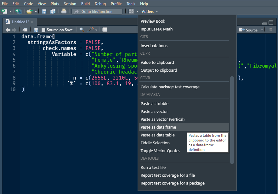
Copy and paste

But manually typing in these values is still tedious and error-prone. Can’t we just copy and paste? Yes we can, with the datapasta package. Install the package:

install.packages('datapasta')

Copy your source table to the clipboard (e.g. from a webpage or Word document) and then select Addins > Paste as (format) into code chunk or script. (I used it to generate the tribble code above!)

Screenshot of the datapasta RStudio addin

Complex kable tables

Functions like kable (Xie 2014) and pander are straightforward to use for simple tables, but do not have many advanced features. For that, try using the package kableExtra (Zhu 2020), which adds just about all the functionality you could ever really need.

Here are some examples.

library(kableExtra)
options(knitr.table.format = 'html')

Add header rows to group columns

kable(my_tbl) %>%
  kable_styling() %>%
  add_header_above(c(' ' = 1, 'Final case-crossover study cohort' = 2))

	Final case-crossover study cohort
Variable	n	%
Number of participants	2658	100.0
Female	2210	83.1
Rheumatoid arthritis	506	19.0
Osteoarthritis	926	34.8
Ankylosing spondylitis	235	8.8
Gout	97	3.6
Arthritis (unspecified)	972	36.6
Fibromyalgia	665	25.0
Chronic headache	271	10.2
Neuropathic pain	371	14.0

Add indents to group rows implicitly

knitr::kable(my_tbl) %>%
  add_indent(c(2, 4), level_of_indent = 1)

Variable	n	%
Number of participants	2658	100.0
Female	2210	83.1
Rheumatoid arthritis	506	19.0
Osteoarthritis	926	34.8
Ankylosing spondylitis	235	8.8
Gout	97	3.6
Arthritis (unspecified)	972	36.6
Fibromyalgia	665	25.0
Chronic headache	271	10.2
Neuropathic pain	371	14.0

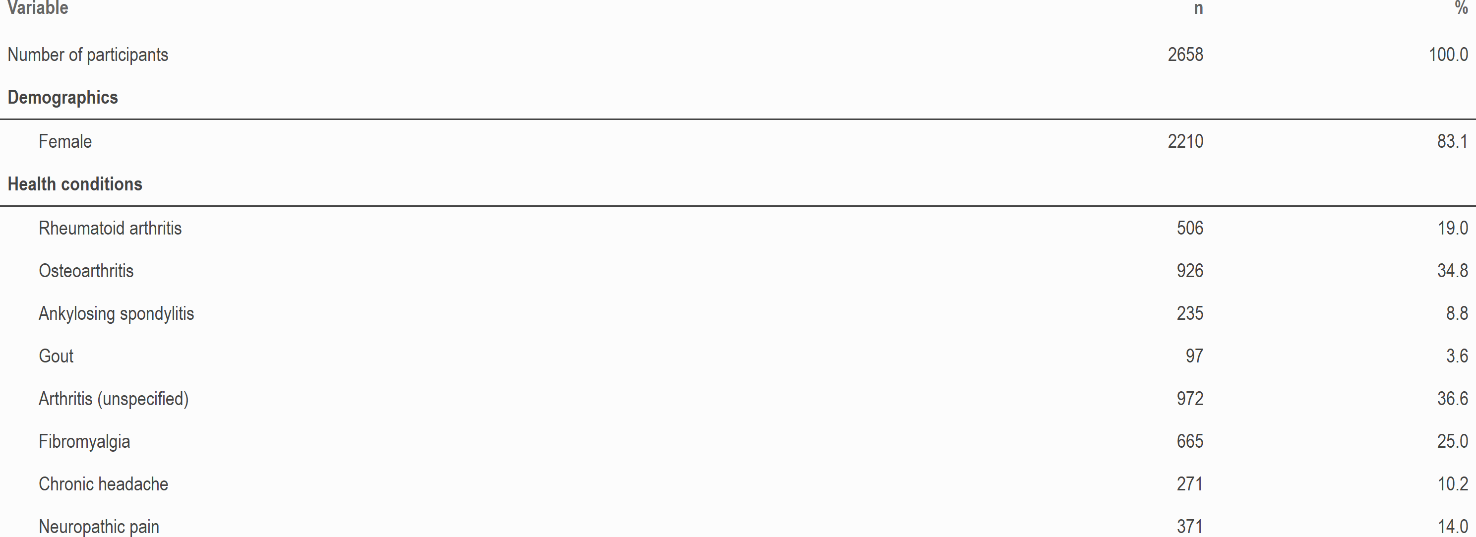
Add labels to group rows explicitly

knitr::kable(my_tbl) %>%
  pack_rows('Demographics', 2, 2) %>%
  pack_rows('Health conditions', 3, 10)

Variable	n	%
Number of participants	2658	100.0
Demographics
Female	2210	83.1
Health conditions
Rheumatoid arthritis	506	19.0
Osteoarthritis	926	34.8
Ankylosing spondylitis	235	8.8
Gout	97	3.6
Arthritis (unspecified)	972	36.6
Fibromyalgia	665	25.0
Chronic headache	271	10.2
Neuropathic pain	371	14.0

Collapse rows that are repeated

kable(engagement_days) %>%
  kable_styling() %>%
  collapse_rows(valign = 'top')

Cluster	Engagement	Min	Q1	Median	Q3	Max
High	Days in study	61	130	203	319	456
	No. days with pain data	4	104	160	254	449
	% days with pain data		73	82	89
Medium	Days in study	22	48	91	182	456
	No. days with pain data	2	26	40	72	311
	% days with pain data		38	52	67
Low	Days in study	2	4	10	21	452
	No. days with pain data	1	2	5	9	64
	% days with pain data		32	56	81
Very Low	Days in study	1	1	1	1	291
	No. days with pain data	1	1	1	1	2
	% days with pain data		100	100	100

library(dplyr)
## Rearrange and sort the columns:
engagement_days %>%
  select(Engagement, Cluster, Min:Max) %>%
  arrange(Engagement, Cluster) %>%
  kable() %>%
  kable_styling %>%
  collapse_rows(valign = 'top')

Engagement	Cluster	Min	Q1	Median	Q3	Max
Days in study	High	61	130	203	319	456
	Medium	22	48	91	182	456
	Low	2	4	10	21	452
	Very Low	1	1	1	1	291
No. days with pain data	High	4	104	160	254	449
	Medium	2	26	40	72	311
	Low	1	2	5	9	64
	Very Low	1	1	1	1	2
% days with pain data	High		73	82	89
	Medium		38	52	67
	Low		32	56	81
	Very Low		100	100	100

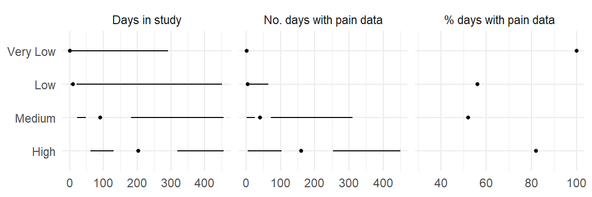
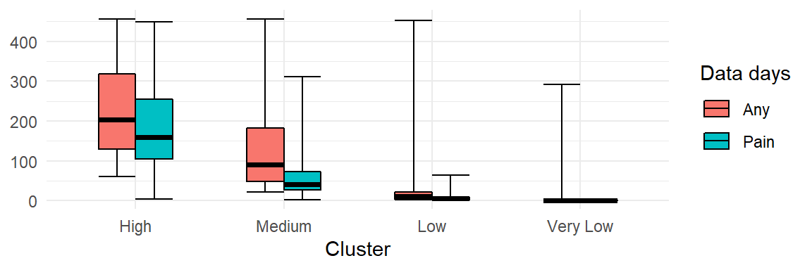
Perhaps clearer representations of the same information:

Add styling

By default, a kableExtra-infused table (a kbl) is unformatted. You can make it look like the default knitr formatting again:

grouped_tbl <-
  kable(my_tbl) %>%
  pack_rows('Demographics', 2, 2) %>%
  pack_rows('Health conditions', 3, 10)

grouped_tbl %>%
  kable_styling()

Variable	n	%
Number of participants	2658	100.0
Demographics
Female	2210	83.1
Health conditions
Rheumatoid arthritis	506	19.0
Osteoarthritis	926	34.8
Ankylosing spondylitis	235	8.8
Gout	97	3.6
Arthritis (unspecified)	972	36.6
Fibromyalgia	665	25.0
Chronic headache	271	10.2
Neuropathic pain	371	14.0

Or better yet, pick from fancier themes and options:

grouped_tbl %>%
  kable_paper(full_width = FALSE)

Variable	n	%
Number of participants	2658	100.0
Demographics
Female	2210	83.1
Health conditions
Rheumatoid arthritis	506	19.0
Osteoarthritis	926	34.8
Ankylosing spondylitis	235	8.8
Gout	97	3.6
Arthritis (unspecified)	972	36.6
Fibromyalgia	665	25.0
Chronic headache	271	10.2
Neuropathic pain	371	14.0

grouped_tbl %>%
  kable_paper('striped', full_width = FALSE)

Variable	n	%
Number of participants	2658	100.0
Demographics
Female	2210	83.1
Health conditions
Rheumatoid arthritis	506	19.0
Osteoarthritis	926	34.8
Ankylosing spondylitis	235	8.8
Gout	97	3.6
Arthritis (unspecified)	972	36.6
Fibromyalgia	665	25.0
Chronic headache	271	10.2
Neuropathic pain	371	14.0

grouped_tbl %>%
  kable_classic('striped', full_width = FALSE)

Variable	n	%
Number of participants	2658	100.0
Demographics
Female	2210	83.1
Health conditions
Rheumatoid arthritis	506	19.0
Osteoarthritis	926	34.8
Ankylosing spondylitis	235	8.8
Gout	97	3.6
Arthritis (unspecified)	972	36.6
Fibromyalgia	665	25.0
Chronic headache	271	10.2
Neuropathic pain	371	14.0

grouped_tbl %>%
  kable_minimal(full_width = FALSE)

Variable	n	%
Number of participants	2658	100.0
Demographics
Female	2210	83.1
Health conditions
Rheumatoid arthritis	506	19.0
Osteoarthritis	926	34.8
Ankylosing spondylitis	235	8.8
Gout	97	3.6
Arthritis (unspecified)	972	36.6
Fibromyalgia	665	25.0
Chronic headache	271	10.2
Neuropathic pain	371	14.0

grouped_tbl %>%
  kable_material('hover')

Variable	n	%
Number of participants	2658	100.0
Demographics
Female	2210	83.1
Health conditions
Rheumatoid arthritis	506	19.0
Osteoarthritis	926	34.8
Ankylosing spondylitis	235	8.8
Gout	97	3.6
Arthritis (unspecified)	972	36.6
Fibromyalgia	665	25.0
Chronic headache	271	10.2
Neuropathic pain	371	14.0

Worried about losing formatting? You can automatically save the resulting table as an image with kableExtra::as_image().

(However, this is not recommended because bitmap screenshots are neither scalable nor searchable and are inaccessible for people with disabilities.)

grouped_tbl %>%
  kable_paper('striped', full_width = T) %>%
  as_image(file = 'table.png', zoom = 3)

Check the documentation for kableExtra to see what else is possible. Results in other formats (such as PDF) may vary.

Best practices for building baseline tables