
One of the reasons to introduce a topological space as a more general structure than a metric space is to be able to define continuous functions without a metric.
Let \(X\), be sets, initially considered without a topological space structure. We write to denote a function with domain and codomain The words function, map, mapping will mean the same thing. The following notation and terminology will be used.
Definition: image of an element, image of a set, preimage of a set
Let be a function. For the element of is the image of under For a subset the subset of defined as
is the image of the set under For a subset the subset of defined as
is called the preimage of the set under
We are now going to define continuity, which does require a topology on both and Attention: we say “ is a topological space” to mean that some topology on is chosen, and open sets are understood to be members of
Definition: continuous function
Let and be topological spaces. A function is continuous if for every subset of open in the preimage is open in
Remark: in MATH21111 Metric Spaces, this was shown to be an equivalent definition of continuity.
This means that when and are metric spaces, considered with their metric topologies, we can use two equivalent definitions of a continuous function:
the - definition of continuity for functions between metric spaces;
the topological definition of continuity, given above.
When or is not a metric space, we do not have the - definition, and can only use the topological definition.
Alert:
Remember, “ is continuous” means open open !
It is not true for a general continuous function that images of open subsets of are open in :
A counterexample is given in the Tutorial.
Proposition: identity functions and constant functions are continuous
Let be topological spaces. The identity map on , defined by for all points is continuous.
Let be a point of The constant function for all (i.e., the function that sends the whole of to one point), is continuous.
Proposition: composition of continuous functions is continuous
Suppose where are topological spaces, and the functions are continuous. Then the composition is also continuous.
It is often useful to characterise continuous functions in terms of closed sets, which we will now define.
Definition: closed set
Let be a topological space. A subset of is closed in if its complement is open in
This definition means that every subset of a topological space falls into one of the four classes:
The last three examples are illustrated by Figure 1.
Alert:
“Not open” does not mean “closed”!
The collection of closed sets in has properties which mirror, but do not repeat, the properties of open sets – we need to exchange unions and intersections:
Proposition: properties of closed sets
If is a topological space, then
Proposition: closed set criterion of continuity
For a function between topological spaces and the following are equivalent:
Proof. Implication 1.2.: assume that is continuous. Let be any closed set in Then is open in Since preimage respects complements (see Tutorial), By continuity of is open, so by definition of “closed”, is closed. We proved that the preimage of every closed set is closed.
Reverse the logic to show 2.1. □
We have arrived at one of the most important definitions of the course.
Definition: homeomorphism, homeomorphic spaces
Let and be topological spaces. A function is a homeomorphism if
Two topological spaces are homeomorphic if there exists a homeomorphism
We will write to indicate that there is a homeomorphism between and or to indicate that is a homeomorphism.
In mathematics, the symbol is typically used to denote an equivalence relation. This is also the case here:
Claim: ‘is homeomorphic to’ is an equivalence relation
‘Is homeomorphic to’ is an equivalence relation between topological spaces.
Proof. We need to check the three axioms of equivalence relation.
Reflexive: we need to show that every space is homeomorphic to itself. Indeed, is a homeomorphism because the identity map is a bijection, the identity map is continuous as shown earlier, and hence the inverse is also continuous.
Symmetric: We need to show that if then Assume that Since is a homeomorphism, the inverse bijection is, by definition, continuous. Furthermore, the inverse of is which is continuous. We conclude that is a homeomorphism.
Transitive: we need to show that if and then Assume that and are homeomorphisms. Then is a homeomorphism: it is a bijection as it has inverse and both and are continuous as compositions of continuous maps. □
Let us now consider examples of homeomorphic spaces. First, introduce a topological space which appears in many examples.
Definition: circle,
The circle is the set
viewed with the topology defined by the Euclidean metric in
Example: some spaces homeomorphic to
Show that the Euclidean line is homeomorphic to the following spaces, viewed with the Euclidean metric:
Solution. We construct pairs of continuous functions which are mutual inverses between some pairs of the given spaces, see Figure 2
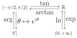
We do not need to construct homeomorphisms between each pair of the given spaces: since “homeomorphic” is an equivalence relation, we have constructed enough to show that all four spaces are homeomorphic to each other.
The homeomorphism between the right half-circle of the unit circle and can be described in purely geometric terms as in Figure 3: take a point of the half-circle and project it onto the vertical tangent line to the half-circle at the point in the plane.
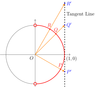
The homeomorphisms shown above are not unique, and there are many other ways of showing that these four spaces are pairwise homeomorphic.
Remark. The four spaces shown above are quite different as metric spaces: for example,
Hence there is no way these metric spaces can be isometric (i.e., equivalent as metric spaces). We thus observe that being homeomorphic (i.e., equivalent as topological spaces) is a weaker requirement, for metric spaces, than being isometric.
The material in this section is not examinable
Knot theory is a branch of mathematics which arose from an attempt to classify knots rigorously by Peter Guthrie Tait (1831–1901). In 1920s, following the work of J. Alexander, knot theory became part of Topology. Since 1980s, knot theory has been applied to the study of DNA and other molecules, and to the study of fluid vortices and has found further applications in Physics.
A knot is a smooth injective function where is the unit circle. The image of the function is a smooth closed curve in which has no self-intersections; such curves are themselves called knots. Two knots are equivalent, or isotopic, if there is a continuous deformation of the space which transforms into
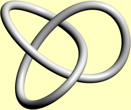
The main problem of knot theory is to classify all knots up to isotopy. For example, a basic result of knot theory is that a trefoil knot, the curve shown in Figure 4, is not isotopic to the unknot (a straightforward copy of the circle in ).
Is the problem of deciding whether two knots are isotopic related to the notion of homeomorphism? After all, every knot is homeomorphic to a circle, isn’t it? Yes, but complements of knots are not homeomorphic. A highly non-obvious result is
Theorem: Gordon-Luecke theorem (1989)
Two knots in are isotopic (up to taking a mirror image) if, and only if, there exists a homeomorphism
The theory of knots extends to links which are unions of disjoint knots in An example of a non-trivial link is the famous Borromean rings: three interlinked circles in such that if any one circle is removed, the remaining two circles become unlinked, see Figure 5. Unlike knots, a link is not determined up to isotopy by a homeomorphism class of its complement.
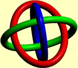
A stylised representation of Borromean rings was chosen as the logo of the International Mathematical Union.
End of non-examinable material.