Model-free estimation of a psychometric function

Example 4. Discrimination of "porthole" views of natural scenes

Xie, Y. & Griffin, L. D. “A 'portholes' experiment for probing perception of small patches of natural images”, Perception, 36, 315, 2007.

MatLab	R

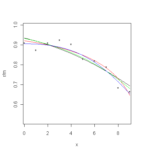
Back to Examples

The subject was presented with a display split into two parts, one containing a pair of patches from the same image, the other a pair from different images, and the subject had to judge which pair came from the same image. The symbols in the figure below show the proportion of correct responses in 200 trials as a function of patch separation.

Parametric and local linear fitting

Three different parametric models and the local linear fitting are used and fits are plotted against the measured psychometric data. Three different parametric models are fitted to these data: Gaussian (probit), Weibull, and reverse Weibull. Local linear fitting is also performed with the bandwidth bwd chosen by the minimising cross-validated deviance.

Load the data and plot the measured psychometric data (black dots):

data("Xie_Griffin") x = Xie_Griffin$x r = Xie_Griffin$r m = Xie_Griffin$m plot( x, r / m, xlim = c( 0.25, 8.76 ), ylim = c( 0.52, 0.99 ), type = "p", pch="*" ) # Limits set to match the MatLab ones

1. For the Gaussian cumulative distribution function (black curve):

val <- binomfit_lims( r, m, x, link = "probit" ) # Plot the fitted curve numxfit <- 199 # Number of new points to be generated minus 1 xfit <- (max(x)-min(x)) * (0:numxfit) / numxfit + min(x) pfit<-predict( val$fit, data.frame( x = xfit ), type = "response" ) lines(xfit, pfit )

2. For the Weibull function (red curve):

val <- binom_weib( r, m, x ) # Plot the fitted curve pfit<-predict( val$fit, data.frame( x = xfit ), type = "response" ) lines(xfit, pfit, col = "red" )

3. For the reverse Weibull function (green curve):

val <- binom_revweib( r, m, x ) # Plot the fitted curve pfit<-predict( val$fit, data.frame( x = xfit ), type = "response" ) lines(xfit, pfit, col = "green" )

4. For the local linear fit (blue curve):

bwd_min <- min( diff( x ) ) bwd_max <- max( x ) - min( x ) bwd <- bandwidth_cross_validation( r, m, x, c( bwd_min, bwd_max ) ) # Plot the fitted curve bwd <- bwd$deviance # choose the estimate based on cross-validated deviance pfit <- locglmfit( xfit, r, m, x, bwd )$pfit lines(xfit, pfit, col = "blue" )

Back to Examples