Model-free estimation of a psychometric function

Example 5. Induction of a visual motion aftereffect

Schofield, A. J., Ledgeway, T., & Hutchinson, C. V. “Asymmetric transfer of the dynamic motion aftereffect between first- and second-order cues and among different second-order cues”, Journal of Vision, 7(8), 1-12, 2007.

MatLab	R

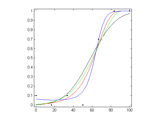
Back to Examples

The subject was presented with a moving adaptation stimulus, followed by a test stimulus. The symbols in the figure below show the proportion of responses in which the subject indicated motion of the test stimulus in the same direction as the adapting stimulus, either up or down, as a function of relative modulation depth. There were 10 trials at each stimulus level.

Parametric and local linear fitting

Three different parametric models and the local linear fitting are used and fits are plotted against the measured psychometric data. Three different parametric models are fitted to these data: Gaussian (probit), Weibull, and reverse Weibull. Local linear fitting is also performed with the bandwidth bwd chosen by the minimising cross-validated deviance.

Load the data and plot the measured psychometric data (black dots):

clear, load examples/Schofield_etal; figure; plot( x, r ./ m, 'k.'); axis([-2 102 -0.02 1.02]); axis square;

1. For the Gaussian cumulative distribution function (black curve):

degpol = 1; % Degree of the polynomial b = binomfit_lims( r, m, x, degpol, 'probit' ); numxfit = 199; % Number of new points to be generated minus 1 xfit = [min(x):(max(x)-min(x))/numxfit:max( x ) ]'; % Plot the fitted curve pfit = binomval_lims( b, xfit, 'probit' ); hold on, plot( xfit, pfit, 'k' );

2. For the Weibull function (red curve):

[ b, K ] = binom_weib( r, m, x, 1, 5 ); guessing = 0; % guessing rate lapsing = 0; % lapsing rate % Plot the fitted curve pfit = binomval_lims( b, xfit, 'weibull', guessing, lapsing, K ); hold on, plot( xfit, pfit, 'r' );

3. For the reverse Weibull function (green curve):

[ b, K ] = binom_revweib( r, m, x ); % Plot the fitted curve pfit = binomval_lims( b, xfit, 'revweibull', guessing, lapsing, K ); hold on, plot( xfit, pfit, 'g' );

4. For the local linear fit (blue curve):

bwd_min = min( diff( x ) ); bwd_max = max( x ) - min( x ); bwd = bandwidth_cross_validation( r, m, x, [ bwd_min, bwd_max ] ); % Plot the fitted curve bwd = bwd(3); % choose the third estimate, which is based on cross-validated deviance pfit = locglmfit( xfit, r, m, x, bwd ); hold on, plot( xfit, pfit, 'b' );

Back to Examples