Model-free estimation of a psychometric function

Example 6. Discrimination of image approximations

Nascimento, S.M.C., Foster, D.H., & Amano, K. “Psychophysical estimates of the number of spectral-reflectance basis functions needed to reproduce natural scenes”, Journal of the Optical Society of America A-Optics Image Science and Vision, 22 (6), 1017-1022, 2005.

MatLab	R

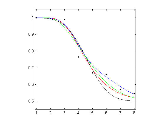
Back to Examples

The subject was shown an image of a natural scene and an approximation of this image based on principal component analysis. The task was to distinguish between the images. The symbols in the figure below show the proportion of correct responses as a function of number of components in the approximation. There were 200 trials at each level pooled over a range of natural scenes.

Parametric and local linear fitting

Three different parametric models and the local linear fitting are used and fits are plotted against the measured psychometric data. Three different parametric models are fitted to these data: Gaussian (probit), Weibull, and reverse Weibull. Local linear fitting is also performed with the bandwidth bwd chosen by the minimising cross-validated deviance.

Load the data and plot the measured psychometric data (black dots), as follows. Notice that in the same example in Żychaluk and Foster (2009) Download PDF, the x-axis was reversed.

clear, load examples/Nascimento_etal; figure; plot( x, r ./ m, 'k.'); axis([0.9 8.1 0.45 1.05]); axis square;

1. For the Gaussian cumulative distribution function (black curve):

degpol = 1; % Degree of the polynomial guessing = 1/2; % guessing rate lapsing = 0; % lapsing rate b = binomfit_lims( r, m, x, degpol, 'probit', guessing, lapsing ); numxfit = 199; % Number of new points to be generated minus 1 xfit = [min(x):(max(x)-min(x))/numxfit:max( x ) ]'; % Plot the fitted curve pfit = binomval_lims( b, xfit, 'probit', guessing, lapsing ); hold on, plot( xfit, pfit, 'k' );

2. For the Weibull function (red curve):

initK = 2; % Initial power parameter in Weibull/reverse Weibull model [ b, K ] = binom_weib( r, m, x, degpol, initK, guessing, lapsing); % Plot the fitted curve pfit = binomval_lims( b, xfit, 'weibull', guessing, lapsing, K ); hold on, plot( xfit, pfit, 'r' );

3. For the reverse Weibull function (green curve):

[ b, K ] = binom_revweib( r, m, x, degpol, initK, guessing, lapsing); % Plot the fitted curve pfit = binomval_lims( b, xfit, 'revweibull', guessing, lapsing, K ); hold on, plot( xfit, pfit, 'g' );

4. For the local linear fit (blue curve):

bwd_min = -min( diff( x ) ); % data is decreasing bwd_max = max( x ) - min( x ); bwd = bandwidth_cross_validation( r, m, x, [ bwd_min, bwd_max ] ); % Plot the fitted curve bwd = bwd(3); % choose the third estimate, which is based on cross-validated deviance pfit = locglmfit( xfit, r, m, x, bwd ); hold on, plot( xfit, pfit, 'b' );

Back to Examples