Model-free estimation of a psychometric function

Example 2. Visual detection of path deviation

Levi, D. M. & Tripathy, S. P. “Is the ability to identify deviations in multiple trajectories compromised by amblyopia?”, Journal of Vision, 6(12), 1367-1379, 2006.

MatLab	R

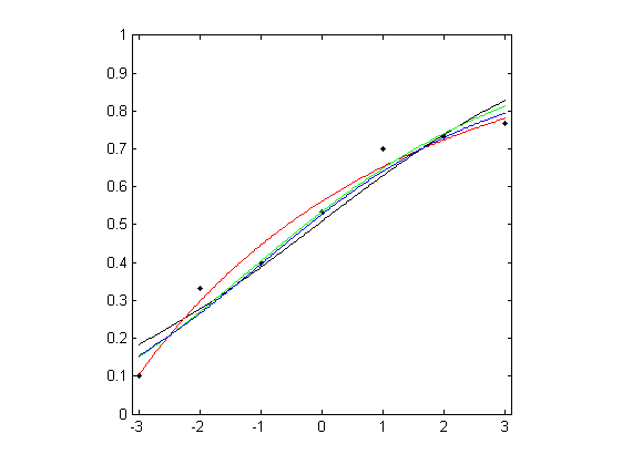
Back to Examples

The subject was presented with the image of a dot moving rightwards on a linear path until it reached the midline of the display, when it changed direction either upwards or downwards. The subject had to indicate the direction. The symbols in the figure below show the proportion of correct responses in 30 trials as the deviation varied from –3 to 3 units.

Parametric and local linear fitting

Three different parametric models and the local linear fitting are used and fits are plotted against the measured psychometric data. Three different parametric models are fitted to these data: Gaussian (probit), Weibull, and reverse Weibull. Local linear fitting is also performed with the bandwidth bwd chosen by the minimising cross-validated deviance.

Load the data and plot the measured psychometric data (black dots):

clear, load examples/Levi_Tripathy; figure; plot( x, r ./ m, 'k.'); axis([-3.1 3.1 0 1]); axis square;

1. For the Gaussian cumulative distribution function (black curve):

degpol = 1; % Degree of the polynomial b = binomfit_lims( r, m, x, degpol, 'probit' ); numxfit = 199; % Number of new points to be generated minus 1 xfit = [min(x):(max(x)-min(x))/numxfit:max( x ) ]'; % Plot the fitted curve pfit = binomval_lims( b, xfit, 'probit' ); hold on, plot( xfit, pfit, 'k' );

2. For the Weibull function (red curve):

[ b, K ] = binom_weib( r, m, x ); guessing = 0; % guessing rate lapsing = 0; % lapsing rate % Plot the fitted curve pfit = binomval_lims( b, xfit, 'weibull', guessing, lapsing, K ); hold on, plot( xfit, pfit, 'r' );

3. For the reverse Weibull function (green curve):

[ b, K ] = binom_revweib( r, m, x ); % Plot the fitted curve pfit = binomval_lims( b, xfit, 'revweibull', guessing, lapsing, K ); hold on, plot( xfit, pfit, 'g' );

4. For the For the local linear fit (blue curve):

bwd_min = min( diff( x ) ); bwd_max = max( x ) - min( x ); bwd = bandwidth_cross_validation( r, m, x, [ bwd_min, bwd_max ] ); % Plot the fitted curve bwd = bwd(3); % Choose the third estimate, which is based on cross-validated deviance pfit = locglmfit( xfit, r, m, x, bwd ); hold on, plot( xfit, pfit, 'b' );

Back to Examples