Model-free estimation of a psychometric function

Example 3. Discrimination of pitch

Unpublished data from S. Carcagno, Lancaster University, July 2008.

MatLab	R

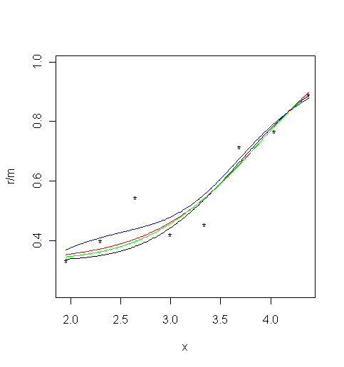
Back to Examples

The subject had to identify the interval containing a tone whose fundamental frequency was different from that in the other two intervals. The symbols in the figure below show the proportion of correct responses as the difference between the tones varied. There were 3–49 trials at each stimulus level.

Parametric and local linear fitting

Three different parametric models and the local linear fitting are used and fits are plotted against the measured psychometric data. Three different parametric models are fitted to these data: Gaussian (probit), Weibull, and reverse Weibull. Local linear fitting is also performed with the bandwidth bwd chosen by the minimising cross-validated deviance.

Load the data and plot the measured psychometric data (black dots):

data("Carcagno") x = Carcagno$x r = Carcagno$r m = Carcagno$m plot( x, r / m, xlim = c( 1.95, 4.35 ), ylim = c( 0.24, 0.99 ), type = "p", pch="*" ) # Limits set to match the MatLab ones

1. For the Gaussian cumulative distribution function (black curve):

guess = 1/3; # guessing rate laps = 0; # lapsing rate val <- binomfit_lims( r, m, x, link = "probit", guessing = guess, lapsing = laps ) numxfit <- 199 # Number of new points to be generated minus 1 xfit <- (max(x)-min(x)) * (0:numxfit) / numxfit + min(x) # Plot the fitted curve pfit<-predict( val$fit, data.frame( x = xfit ), type = "response" ) lines(xfit, pfit )

2. For the Weibull function (red curve):

val <- binom_weib( r, m, x, guessing = guess, lapsing = laps ) # Plot the fitted curve pfit<-predict( val$fit, data.frame( x = xfit ), type = "response" ) lines(xfit, pfit, col = "red" )

3. For the reverse Weibull function (green curve):

val <- binom_revweib( r, m, x, guessing = guess, lapsing = laps ) # Plot the fitted curve pfit<-predict( val$fit, data.frame( x = xfit ), type = "response" ) lines(xfit, pfit, col = "green" )

4. For the local linear fit (blue curve):

bwd_min <- min( diff( x ) ) bwd_max <- max( x ) - min( x ) bwd <- bandwidth_cross_validation( r, m, x, c( bwd_min, bwd_max ) ) # Plot the fitted curve bwd <- bwd$deviance # choose the estimate based on cross-validated deviance pfit <- locglmfit( xfit, r, m, x, bwd )$pfit; lines(xfit, pfit, col = "blue" )

Back to Examples