Tutorial on Colour Information

Tutorial on Estimating Information from Image Colours

This page provides an introduction to estimating Shannon information from RGB coloured images and how these estimates may be used in practice.

1. Basics

The colors in an image of a scene provide information about its reflecting surfaces under the prevailing illumination. But how should this information be quantified? How does it vary from scene to scene? And how does it depend on the spectral sensitivities of the camera or eye used to view the scene? The aim of this tutorial is to show how these questions can be addressed with the aid of some basic ideas from information theory and the computational routines downloadable from this site.

You will need this package, which contains MatLab MEX files for Windows 7 MatLab 32 bit, Windows 7 MatLab 64 bit, and Mac OSX operating systems. For Windows 10, you will need the updated routines in this package.

This material is base on the following publication: Marín-Franch, I. and Foster, D. H. (2013). Estimating Information from Image Colors: An Application to Digital Cameras and Natural Scenes. IEEE Transactions on Pattern Analysis and Machine Intelligence, 35(1), 78-91.

Suppose that a camera or the eye produces a triplet of values r, g, b at each point of the image, as in Fig. 1.

brufefields

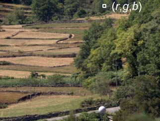
Figure 1. Fields scene. The pixel at the top right has colour values r, g, b.

If the location of the point is unpredictable, then taken together, the triplet (r, g, b) can be treated as a trivariate continuous random variable, A say, with probability density function (pdf), f say. Histogram representations of the r, g, b signal levels (for the eye, long-, medium-, short-wavelength cone signal levels) are shown in Fig. 2.

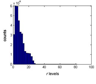
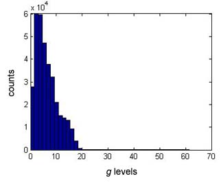
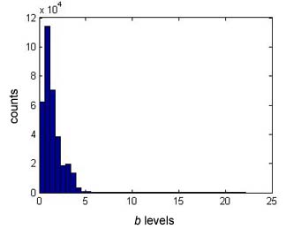
Figure 2. Histograms of estimated r, g, b signal levels from Fig. 1 for the human eye.

The uncertainty or randomness of the variable A is captured by Shannon's differential entropy h(A), defined [1] as

h(A) = − ∫ f(a) log f(a) da.

(1)

The entropy is measured in bits if the logarithm in Eqn (1) is to the base 2.

The mutual information I(A₁;A₂) between two images of a scene under different conditions, e.g. under different illuminations, represents how much information one scene contains about the other by virtue of its colours. It can be defined by the following combination of entropies [1]:

I(A₁;A₂) = h(A₁) + h(A₂) − h(A₁,A₂),

(2)

where h(A₁,A₂) is the differential entropy of the variables A₁ and A₂. Unlike differential entropy, mutual information does not depend on the units used to quantify the r, g, b signal levels. As explained in the next section, mutual information is intimately related to the number of identifiable points in a scene. These estimates do not include any uncertainty in the camera or eye due to noise, whose differential entropy may also be included in the calculation [2]. Different cameras with different sensors will produce different histograms from those illustrated in Fig. 2. Examples are given in [3].

Notice that these calculations are based solely on spectral information. They make no use of information about spatial position.

2. Kozachenko-Leonenko estimator and offset versions

Mutual information depends directly or indirectly on probability density functions. Unfortunately, using histograms such as those in Fig. 2 to estimate pdfs is difficult and can lead to marked biases [4]. Instead, it is possible to use nearest-neighbour statistics to estimate entropies directly from the data, and then apply Eqn (2) to estimate mutual information. The Kozachenko-Leonenko kth-nearest-neighbour estimator [5] is used here. Its convergence properties were improved with an offset device, details of which are given in [6].

Shannon's channel coding theorem [2] gives a nice interpretation of the mutual information between two images of a scene obtained under two different illuminations conditions. If the mutual information is I, then the number of points or elements in the scene that retain their identity by virtue of their colour is given by

N = 2^I.

As an example, the images in Fig. 3 are of the scene shown in Fig. 1 under the setting sun and north skylight.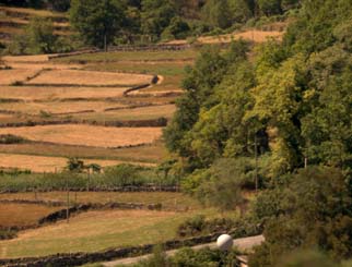

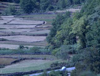
brufefields 4000 K brufefields 25000 K

Figure 3. Images of the scene shown in Fig. 1 under the setting sun (left) and north skylight (right), correlated colour temperatures of 4000 K and 25000 K, respectively.

For the human eye, the offset Kozachenko-Leonenko estimator of the mutual information between these two images is 17.0 bits and the number of identifiable points is 1.3x10⁵.

The following sections describe how to make these kinds of estimates with the routines available in the package downloadable here and updated here.

3. Contents of the package

The package contains MatLab MEX files for Windows 7 MatLab 32 bit, Windows 7 MatLab 64 bit, and Mac OSX operating systems, and it can be downloaded here. With the MatLab MEX files, both differential entropy and mutual information can be calculated. The C++ source code used to generate the MEX files is also included in the package.

For Windows 10, updated routines for differential entropy and mutual information can be downloaded here.

The C++ code for the MatLab MEX files was implemented by Martin Sanz (martin.sanz@uv.es).

If you use this software in published research, please give the reference of the source work in full, namely Marín-Franch, I. and Foster, D. H. (2013). Estimating Information from Image Colors: An Application to Digital Cameras and Natural Scenes. IEEE Transactions on Pattern Analysis and Machine Intelligence, 35(1), 78-91.

This tutorial uses hyperspectral reflectance images so that changes in reflectance spectra can be accurately calculated under changes in illuminant. A small test hyperspectral image is included in the package. If you want to experiment with other, larger, hyperspectral images, then sets of reflectance files are available here and here and separate, larger sets of radiance files are available here and here. With some hyperspectral images, the edges may need trimming to remove pixels with zero or padded values that were introduced during postprocessing.

These hyperspectral images are also available from the University of Minho.

4. Using the package to estimate mutual information between two images

To estimate the mutual information between the distributions of colours in two images, proceed as follows. Load the subsampled scene ref4_scene5.mat and find the dimensions of the loaded array reflectances.

 load ref4_scene5.mat;

[nrow,ncol,nwav] = size(reflectances);

The number of rows nrow should be 255, the number of columns ncol 335, and the number of wavelengths nwav 33.

Next obtain the radiances of the reflected image of the scene under a daylight illuminant of color-correlated temperature 25000 K and then one of 4000 K (a for-loop is less efficient than MATLAB's bsxfun function, but it makes little difference here).

 load illum_25000.mat;

load illum_4000.mat;

radiances_25000 = zeros(nrow,ncol,nwav); % initialize array

radiances_4000 = zeros(nrow,ncol,nwav); % initialize array

for i = 1:33,

  radiances_25000(:,:,i) =
reflectances(:,:,i)*illum_25000(i);

  radiances_4000(:,:,i) =
reflectances(:,:,i)*illum_4000(i);

end

To obtain the RGB sensor responses of a camera, choose one of the following sensor sets: agilent, foveonx3, kodak, nikond1, and sony.

rgbsens = rgbcurves('agilent

');

rgbsens(:,1) = []; % delete first column with wavelengths

radiances_25000 = reshape(radiances_25000,nrow*ncol,nwav );

radiances_4000 = reshape(radiances_4000,nrow*ncol,nwav );

rgb_25000 = radiances_25000*rgbsens;

rgb_4000 = radiances_4000*rgbsens;

To estimate the mutual information apply the Kozachenko-Leonenko estimator 'kl' and, for comparison, the offset version of the estimator 'klo' to the arrays rgb_25000 and rgb_4000.

 mi = mikl(rgb_25000,rgb_4000,'kl' );

mio = mikl(rgb_25000,rgb_4000,'klo');

The Kozachenko-Leonenko estimator gives a value of 13.9 bits whereas the offset estimator gives a value of 17.2 bits.

The calculation can be repeated with any of the other sensor sets to illustrate the effect of their different spectral sensitvities. For example, replace 'agilent' by 'eye' to obtain the following:

rgbsens = rgbcurves('eye

');

rgbsens(:,1) = []; % delete first column with wavelengths

radiances_25000 = reshape(radiances_25000,nrow*ncol,nwav );

radiances_4000 = reshape(radiances_4000,nrow*ncol,nwav );

rgb_25000 = radiances_25000*rgbsens;

rgb_4000 = radiances_4000*rgbsens;

      mi =
mikl(rgb_25000,rgb_4000,'kl' );

mio = mikl(rgb_25000,rgb_4000,'klo');

The Kozachenko-Leonenko estimator gives a value of 13.0 bits and the offset estimator gives a value of 16.9 bits.

The value of 16.9 bits for the offset estimator is only slightly smaller than the 17.0 bits reported in Section 2, which was derived from an image with higher spatial resolution (downloadable as a zip file here).

5. Using the package to estimate differential entropies

The estimate of the mutual information in Section 4 is based on Eqn (2). The individual estimates of the differential entropies can be obtained explicitly as follows:

h1 =
entkl(rgb_25000,'klo');

h2 = entkl(rgb_4000,'klo');

      h12 = entkl([rgb_25000,rgb_4000],'klo');

The estimates are 4.2 bits, 3.1 bits, and -9.6 bits, respectively. When combined according to Eqn (2), they give the estimate of 16.9 bits for the mutual information, as in Section 4.

6. Citing

7. Other applications and hyperspectral imaging in color vision research

Reference [7] provides more examples of the use of differential entropy and mutual information in colour vision research. These include estimates of the effective colour gamut volume, the number of discriminable surfaces, and the frequency and magnitude of metamerism and generalized metamerism. Figure 4 in Reference [7] shows the scene with the greatest number of discriminable surfaces. A colour rendering of the scene is provided below:

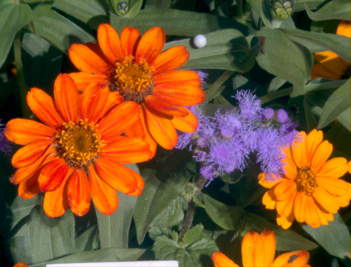
A hyperspectral radiance image of this scene, 'sfum1', is available here as a zipped Matlab file, size 1024 x 1344 x 33, with spectral radiance in W m⁻² sr⁻¹ nm⁻¹.

Other images are available elsewhere on this site and at the University of Minho.

For a more general introduction to hyperspectral imaging and its uses in human color vision research, see Reference [8]. It describes several example applications. These include calculating the color properties of scenes such as gamut volume and metamerism, and analyzing the utility of color in observer tasks such as identifying surfaces under illuminant changes. These analyses draw on calculations of differential entropy and mutual information similar to those outlined here.

References

T. Cover, T. M., & Thomas, J. A. (2006). Elements of Information Theory (2nd ed.). Hoboken, New Jersey: John Wiley & Sons, Inc.

Marín-Franch, I. and Foster, D. H. (2010). Number of perceptually distinct surface colors in natural scenes. Journal of Vision, 10(9):9(9).

Foster, D. H. and Marín-Franch, I. (2013). Effectiveness of Digital Camera Sensors in Distinguishing Colored Surfaces in Outdoor Scenes. Imaging Systems and Applications, Arlington, Virginia, http://dx.doi.org/10.1364/ISA.2013.ITh3D.2
Steuer, R., Kurths, J., Daub, C. O., Weise, J., and Selbig, J. (2002). The mutual information: Detecting and evaluating dependencies between variables. Bioinformatics, 18, S231-S240.
Kozachenko, L. F. and Leonenko, N. N. (1987). Sample estimate of the entropy of a random vector. Problems of Information Transmission (Tr. Problemy Peredachi Informatsii. Vol. 23, No.2, pp. 9-16, 1987), 23(2), 95-101.

Marín-Franch, I. and Foster, D. H. (2013). Estimating Information from Image Colors: An Application to Digital Cameras and Natural Scenes. IEEE Transactions on Pattern Analysis and Machine Intelligence, 35(1), 78-91.
Foster, D.H. (2018). The Verriest Lecture: Color vision in an uncertain world. Journal of the Optical Society of America A, 35, B192-B201. https://doi.org/10.1364/JOSAA.35.00B192. [download PDF here]
Foster, D.H. and Amano, K. (2019). Hyperspectral imaging in color vision research: tutorial. Journal of the Optical Society of America A, 36, 606-627. https://doi.org/10.1364/JOSAA.36.000606 . [download PDF here]

A Concise Guide to Communication in Science & Engineering

		How to write research articles, literature reviews, technical reports, dissertations and theses How to deal with mathematical material, statistical inference, data fitting, plotting graphs How to submit papers for publication, measure impact, present posters, give lectures and talks How to handle ethical issues, manage data, avoid plagiarism The advice in this guide is based on several hundred sources. It includes practical checklists at the ends of chapters for quick reference and verification, and it has over 400 examples of good and bad scientific writing and graphing from published research articles.
Published by Oxford University Press, November 2017, 408 pages. ISBN: 9780198704249. Available as hardback, paperback, or ebook.

d.h.foster@manchester.ac.uk | +44 (0)161 306 3888 | www.eee.manchester.ac.uk/d.h.foster
Department of Electrical and Electronic Engineering, University of Manchester, Manchester M13 9PL, UK